吴川网站建设云南省建设厅官方网站证书

1写在前面

前面我们用WGCNA分析得到多个模块，其中有一些模块和我们感兴趣的表型或者临床特征是相关的。🥳

接着就是要做模块的富集分析了，帮助我们了解这些模块的基因都有哪些已知的功能，涉及到哪些通路，在哪些疾病中最为重要。🥰

现在这种做富集分析的包还是蛮多的，WGCNA包内也是内置了相关功能，不过首推的还是Y叔的clusterProfiler，在我心中真是YYDS。🫶

2用到的包

rm(list = ls())
library(WGCNA)
library(tidyverse)
library(clusterProfiler)
library(enrichplot)
library(org.Mm.eg.db)

3示例数据

load("FemaleLiver-01-dataInput.RData")
load("FemaleLiver-02-networkConstruction-auto.RData")

4整理富集分析的输入文件

一些不会使用代码的小伙伴可以采用将基因列表放到一些在线的网站上去做富集分析，如:👇

• http://www.metascape.org/
• http://kobas.cbi.pku.edu.cn/

4.1 整理文件

annot <-  read.csv(file = "./FemaleLiver-Data/GeneAnnotation.csv");
probes <-  names(datExpr)
probes2annot <-  match(probes, annot$substanceBXH)
allLLIDs <-  annot$LocusLinkID[probes2annot];
intModules <-  c("brown", "red", "salmon")

4.2 循环输出文件

这里你就可以获得你感兴趣模块的genelist了，去在线网站做富集分析吧。🤠

for (module in intModules){
  modGenes <-  (moduleColors==module)
  modLLIDs <-  allLLIDs[modGenes]
  fileName <-  paste("LocusLinkIDs-", module, ".txt", sep="")
  write.table(as.data.frame(modLLIDs), file = fileName, row.names = F, col.names = F)
  }

5内置函数进行富集分析

WGCNA包内也内置了分析函数，可以直接调用。😙

5.1 GO富集分析

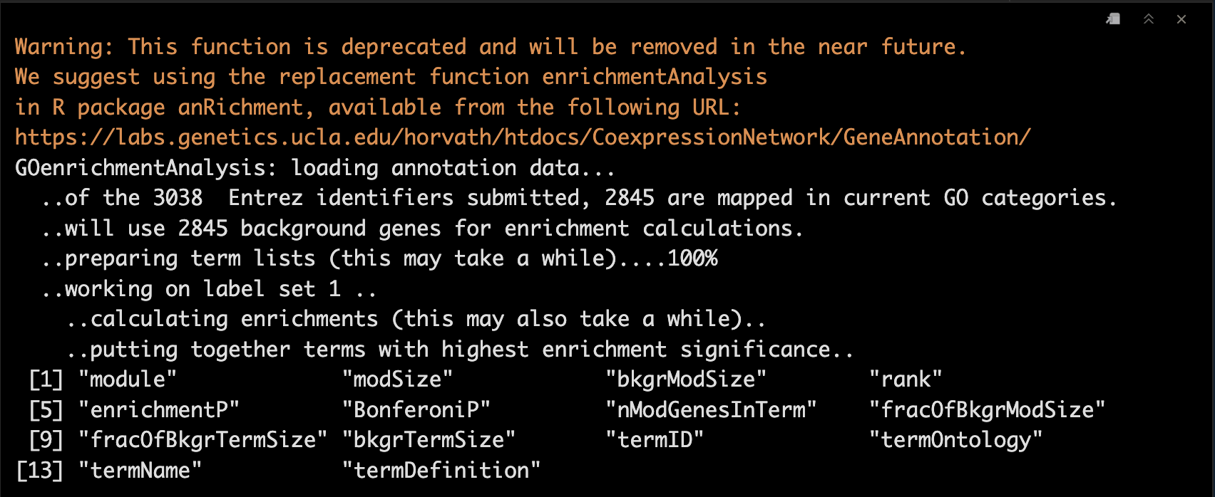
GOenr <-  GOenrichmentAnalysis(moduleColors, allLLIDs, organism = "mouse", nBestP = 10);

tab <-  GOenr$bestPTerms[[4]]$enrichment

names(tab)

write.table(tab, file = "GOEnrichmentTable.csv", sep = ",", quote = TRUE, row.names = FALSE)

5.2 查看结果

keepCols <-  c(1, 2, 5, 6, 7, 12, 13)
screenTab <-  tab[, keepCols]
numCols <-  c(3, 4)
screenTab[, numCols] <-  signif(apply(screenTab[, numCols], 2, as.numeric), 2)
screenTab[, 7] <-  substring(screenTab[, 7], 1, 40)
colnames(screenTab) = c("module", "size", "p-val", "Bonf", "nInTerm", "ont", "term name");
rownames(screenTab) = NULL;
options(width=95)
screenTab

6clusterProfiler包进行富集分析

我们再补充一个Y叔的神包clusterProfiler包进行富集分析的方法，也是我个人最推荐的。🥰

6.1 整理输入文件

这里我们假设我们感兴趣的模块是salmon, red, brown, 我们用一下compareCluster函数，将他们都展示在一张图上。🤨

salmon <- allLLIDs[moduleColors == "salmon"] %>% 
  na.omit()

red <- allLLIDs[moduleColors == "red"]%>% 
  na.omit()

brown <- allLLIDs[moduleColors == "brown"]%>% 
  na.omit()

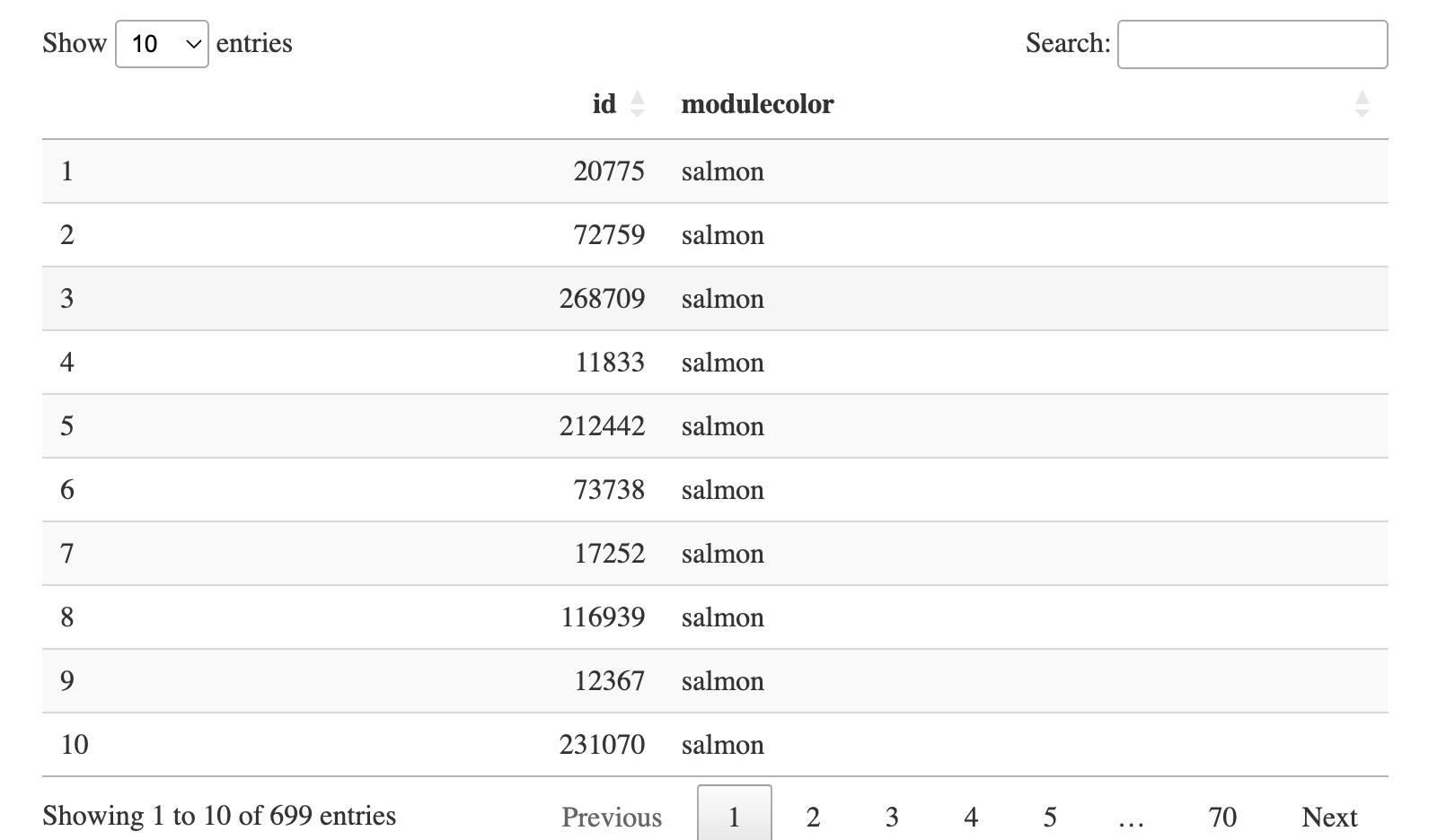
three_modules <- data.frame(id = c(salmon, red, brown),
                            modulecolor = rep(c("salmon", "red", "brown"), 
                                                      c(length(salmon), 
                                                        length(red),
                                                        length(brown))
                                                      )
                            )
DT::datatable(three_modules)

6.2 GO富集分析

其实不光可以做GO富集分析，KEGG, Reactome， GSEA等都是可以的，看大家自己的需求吧。🤩

formula_res.GO <- compareCluster(data = three_modules, 
                              id~modulecolor, 
                              fun="enrichGO",
                              OrgDb = 'org.Mm.eg.db')

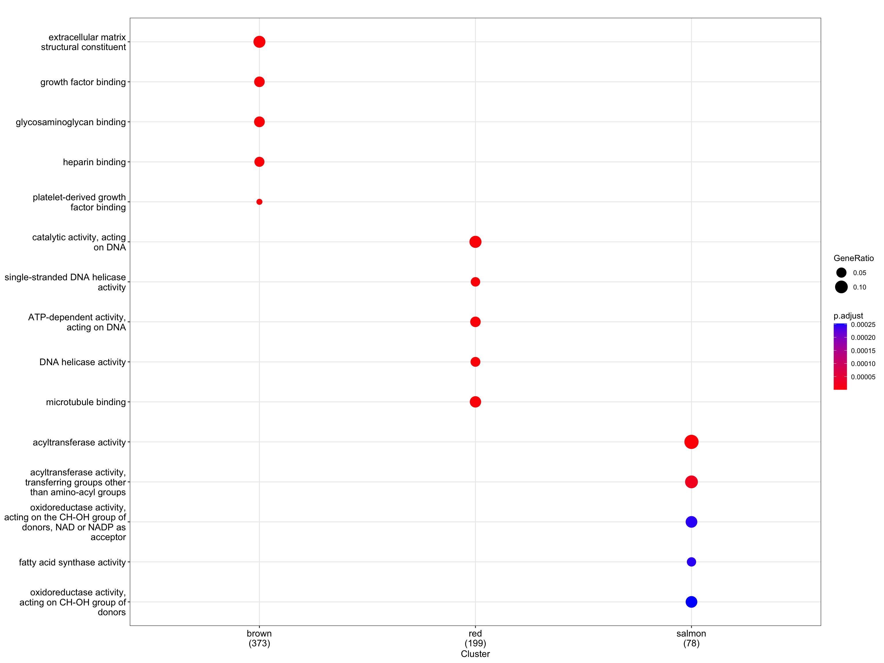
6.3 dotplot展示富集结果

Y叔写了几种可视化的方式，不做具体介绍了，大家自己喜欢什么样的就弄成什么样吧，颜色也是配成你的心头好就行。😏

dotplot(formula_res.GO)

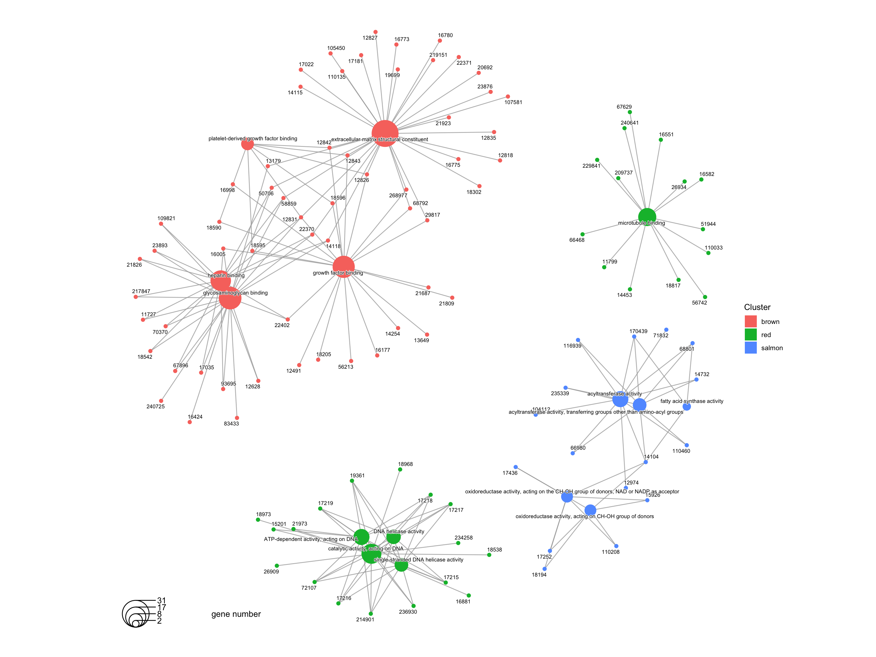
6.4 cnetplot展示富集结果

这种方式展示也不错，大家可以试试。🤪

cnetplot(formula_res.GO)

7如何引用

📍
Langfelder, P., Horvath, S. WGCNA: an R package for weighted correlation network analysis. BMC Bioinformatics 9, 559 (2008). https://doi.org/10.1186/1471-2105-9-559

点个在看吧各位~ ✐.ɴɪᴄᴇ ᴅᴀʏ 〰