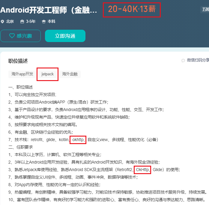
当前位置: 首页 > news >正文

酒店网站建设 源码wordpress改微博系统

酒店网站建设 源码,wordpress改微博系统,网站qq在线状态,佛山做外贸网站哪家好🍨 本文为🔗365天深度学习训练营 中的学习记录博客🍖 原作者:K同学啊 SVM与集成学习 SVMSVM线性模型SVM非线性模型SVM常用参数 集成学习随机森林导入数据查看数据信息数据分析随机森林模型预测结果结果分析 个人总结 SVM 超平面&…
  • 🍨 本文为🔗365天深度学习训练营 中的学习记录博客
  • 🍖 原作者:K同学啊

SVM与集成学习

  • SVM
    • SVM线性模型
    • SVM非线性模型
    • SVM常用参数
  • 集成学习
  • 随机森林
    • 导入数据
    • 查看数据信息
    • 数据分析
    • 随机森林模型
    • 预测结果
    • 结果分析
  • 个人总结

SVM

  • 超平面:SVM 在特征空间中寻找一个能够最大化类别间隔的超平面,称为最大间隔超平面。这个超平面就是将数据集分成不同类别的边界。
  • 支持向量:支持向量是离分隔超平面最近的样本点,它们决定了超平面的位置和方向。换句话说,只有这些样本对分类结果有影响,其他的样本点则不影响。

SVM线性模型

from sklearn import datasets
from sklearn.model_selection import train_test_split
from sklearn.preprocessing import StandardScaler
from sklearn.svm import SVC
from sklearn.metrics import accuracy_score# 加载数据集
iris = datasets.load_iris()
X = iris.data
y = iris.target# 数据预处理
sc = StandardScaler()
X = sc.fit_transform(X)# 训练集和测试集的分割
X_train, X_test, y_train, y_test = train_test_split(X, y, test_size=0.3, random_state=42)# 创建SVM模型
svm = SVC(kernel='linear', C=1.0)# 训练模型
svm.fit(X_train, y_train)# 预测
y_pred = svm.predict(X_test)# 评估模型性能
accuracy = accuracy_score(y_test, y_pred)
print('Accuracy: %.2f' % (accuracy * 100.0))

SVM非线性模型

from sklearn import datasets
from sklearn.model_selection import train_test_split
from sklearn.preprocessing import StandardScaler
from sklearn.svm import SVC
from sklearn.metrics import accuracy_score# 加载数据集
iris = datasets.load_iris()
X = iris.data
y = iris.target# 数据预处理
sc = StandardScaler()
X = sc.fit_transform(X)# 训练集和测试集的分割
X_train, X_test, y_train, y_test = train_test_split(X, y, test_size=0.3, random_state=42)# 创建SVM模型
svm = SVC(kernel='rbf', C=1.0, gamma=0.1)# 训练模型
svm.fit(X_train, y_train)# 预测
y_pred = svm.predict(X_test)# 评估模型性能
accuracy = accuracy_score(y_test, y_pred)
print('Accuracy: %.2f' % (accuracy * 100.0))

SVM常用参数

  1. C(默认值:1.0)
    ○ 作用:惩罚参数,用于平衡最大化分类间隔和误分类惩罚之间的关系。
    ○ 解释:较大的 C 值意味着对误分类的惩罚更大,模型会倾向于将更多的训练数据点分类正确,但可能会导致间隔变小,可能出现过拟合;较小的 C 值则会更关注于间隔的大小,而允许更多的误分类,从而提高模型的泛化能力。
    ○ 常用范围:通常在 0.001 到 1000 之间进行调节。
  2. kernel(默认值:‘rbf’)
    ○ 作用:指定要使用的核函数,支持不同的非线性映射方法。
    ○ 可选值:
    ■ ‘linear’:线性核函数,即不进行任何非线性映射。
    ■ ‘poly’:多项式核函数,通常用于多项式可分的情况。
    ■ ‘rbf’:径向基函数(Radial Basis Function),又称高斯核,是最常用的非线性核函数。
    ■ ‘sigmoid’:类似于神经网络的激活函数,较少使用。
    ■ 你也可以传递自定义核函数,方法是传递一个函数。
  3. degree (默认值:3)
    ○ 作用:当 kernel=‘poly’ 时,指定多项式核的多项式次数。
    ○ 解释:如果使用多项式核函数(poly),degree 参数决定多项式的阶数,通常是 2 或 3。
  4. gamma(默认值:‘scale’)
    ○ 作用:核函数系数,适用于 ‘rbf’、‘poly’ 和 ‘sigmoid’ 核函数。
    ○ 可选值:
    ■ ‘scale’:使用 1 / (n_features * X.var()) 作为默认值。这个值会根据输入特征的数量和方差自动调整。
    ■ ‘auto’:使用 1 / n_features 作为值。
    ○ 解释:gamma 值越大,模型越倾向于拟合训练数据,但可能会导致过拟合;gamma 值越小,模型更倾向于平滑。
  5. coef0(默认值:0.0)
    ○ 作用:核函数中的独立项,仅在 kernel=‘poly’ 或 kernel=‘sigmoid’ 时有意义。
    ○ 解释:用于控制多项式核函数和 sigmoid 核函数中的偏移量。

集成学习

  1. Bagging在做预测时,对于分类任务,使用简单的投票法。对于回归任务使用简单平均法。若分类预测时出现两个类票数一样时,则随机选择一个。
  2. Boosting 工作原理:
  • 弱学习器:中的弱学习器通常是性能稍微优于随机猜测的模型,通常使用简单的模型(如浅层决策树)。
  • 加权训练:在每一次迭代中,Boosting 会调整每个样本的权重,增加那些前一次模型预测错误样本的权重,使得后续的学习器更关注这些难以分类的样本。
  • 加权投票:最终模型是通过将所有弱学习器的预测结果加权整合而成,通常采用加权投票(分类问题)或加权平均(回归问题)。

随机森林

  • 一种基于集成学习的算法,主要用于分类和回归分析。随机森林通过结合多个决策树来提高模型的准确性和稳健性,步骤如下:
  1. 随机抽样:从原始训练数据中随机抽取多个样本集(通常是相同大小),为每棵决策树准备训练数据。
  2. 构建决策树:对于每个样本集,根据随机选取的特征构建一棵决策树。树的生长过程中使用信息增益、基尼指数等标准进行节点分裂。
  3. 集成预测:
    对于分类任务,随机森林通过对所有决策树的预测进行投票,选择票数最多的类别作为最终类别。
    对于回归任务,计算所有树的预测值的平均值。

导入数据

import pandas as pd
import numpy as np
import seaborn as sns
from sklearn.preprocessing import LabelEncoder
from sklearn.model_selection import train_test_split
from sklearn.ensemble import RandomForestClassifier
from sklearn.metrics import classification_reportdata = pd.read_csv(r'C:\Users\11054\Desktop\kLearning\L678_learning\data.csv')
data

查看数据信息

data.info()
import matplotlib.pyplot as pltplt.rcParams['font.family'] = 'SimHei'  # 指定默认字体为黑体
feature_map = {'Temperature': '温度','Humidity': '湿度百分比','Wind Speed': '风速','Precipitation (%)': '降水量百分比','Atmospheric Pressure': '大气压力','UV Index': '紫外线指数','Visibility (km)': '能见度'
}
plt.figure(figsize=(15, 10))for i, (col, col_name) in enumerate(feature_map.items(), 1):plt.subplot(2, 4, i)sns.boxplot(y=data[col])plt.title(f'{col_name}的箱线图', fontsize=14)plt.ylabel('数值', fontsize=12)plt.grid(axis='y', linestyle='--', alpha=0.7)plt.tight_layout()
plt.show()
C:\Users\11054\AppData\Local\Temp\ipykernel_7496\1699620420.py:22: UserWarning: Glyph 8722 (\N{MINUS SIGN}) missing from current font.plt.tight_layout()
C:\Users\11054\.conda\envs\kmate\lib\site-packages\IPython\core\pylabtools.py:152: UserWarning: Glyph 8722 (\N{MINUS SIGN}) missing from current font.fig.canvas.print_figure(bytes_io, **kw)

在这里插入图片描述

print(f"温度超过60°C的数据量:{data[data['Temperature'] > 60].shape[0]},占比{round(data[data['Temperature'] > 60].shape[0] / data.shape[0] * 100,2)}%。")
print(f"湿度百分比超过100%的数据量:{data[data['Humidity'] > 100].shape[0]},占比{round(data[data['Humidity'] > 100].shape[0] / data.shape[0] * 100,2)}%。")
print(f"降雨量百分比超过100%的数据量:{data[data['Precipitation (%)'] > 100].shape[0]},占比{round(data[data['Precipitation (%)'] > 100].shape[0] / data.shape[0] * 100,2)}%。")
温度超过60°C的数据量:207,占比1.57%。
湿度百分比超过100%的数据量:416,占比3.15%。
降雨量百分比超过100%的数据量:392,占比2.97%。

数据分析

data.describe(include='all')
plt.figure(figsize=(20, 15))
plt.subplot(3, 4, 1)
sns.histplot(data['Temperature'], kde=True,bins=20)
plt.title('温度分布')
plt.xlabel('温度')
plt.ylabel('频数')plt.subplot(3, 4, 2)
sns.boxplot(y=data['Humidity'])
plt.title('湿度百分比箱线图')
plt.ylabel('湿度百分比')plt.subplot(3, 4, 3)
sns.histplot(data['Wind Speed'], kde=True,bins=20)
plt.title('风速分布')
plt.xlabel('风速(km/h)')
plt.ylabel('频数')plt.subplot(3, 4, 4)
sns.boxplot(y=data['Precipitation (%)'])
plt.title('降雨量百分比箱线图')
plt.ylabel('降雨量百分比')plt.subplot(3, 4, 5)
sns.countplot(x='Cloud Cover', data=data)
plt.title('云量 (描述)分布')
plt.xlabel('云量 (描述)')
plt.ylabel('频数')plt.subplot(3, 4, 6)
sns.histplot(data['Atmospheric Pressure'], kde=True,bins=10)
plt.title('大气压分布')
plt.xlabel('气压 (hPa)')
plt.ylabel('频数')plt.subplot(3, 4, 7)
sns.histplot(data['UV Index'], kde=True,bins=14)
plt.title('紫外线等级分布')
plt.xlabel('紫外线指数')
plt.ylabel('频数')plt.subplot(3, 4, 8)
Season_counts = data['Season'].value_counts()
plt.pie(Season_counts, labels=Season_counts.index, autopct='%1.1f%%', startangle=140)
plt.title('季节分布')plt.subplot(3, 4, 9)
sns.histplot(data['Visibility (km)'], kde=True,bins=10)
plt.title('能见度分布')
plt.xlabel('能见度(Km)')
plt.ylabel('频数')plt.subplot(3, 4, 10)
sns.countplot(x='Location', data=data)
plt.title('地点分布')
plt.xlabel('地点')
plt.ylabel('频数')plt.subplot(3, 4, (11,12))
sns.countplot(x='Weather Type', data=data)
plt.title('天气类型分布')
plt.xlabel('天气类型')
plt.ylabel('频数')plt.tight_layout()
plt.show()
C:\Users\11054\AppData\Local\Temp\ipykernel_7496\3587563545.py:65: UserWarning: Glyph 8722 (\N{MINUS SIGN}) missing from current font.plt.tight_layout()
C:\Users\11054\.conda\envs\kmate\lib\site-packages\IPython\core\pylabtools.py:152: UserWarning: Glyph 8722 (\N{MINUS SIGN}) missing from current font.fig.canvas.print_figure(bytes_io, **kw)

在这里插入图片描述

随机森林模型

new_data = data.copy()
label_encoders = {}
categorical_features = ['Cloud Cover', 'Season', 'Location', 'Weather Type']
for feature in categorical_features:le = LabelEncoder()new_data[feature] = le.fit_transform(data[feature])label_encoders[feature] = lefor feature in categorical_features:print(f"'{feature}'特征的对应关系:")for index, class_ in enumerate(label_encoders[feature].classes_):print(f"  {index}: {class_}")
'Cloud Cover'特征的对应关系:0: clear1: cloudy2: overcast3: partly cloudy
'Season'特征的对应关系:0: Autumn1: Spring2: Summer3: Winter
'Location'特征的对应关系:0: coastal1: inland2: mountain
'Weather Type'特征的对应关系:0: Cloudy1: Rainy2: Snowy3: Sunny
# 构建x,y
x = new_data.drop(['Weather Type'],axis=1)
y = new_data['Weather Type']# 划分数据集
x_train,x_test,y_train,y_test = train_test_split(x,y,test_size=0.3,random_state=15)# 构建随机森林模型
rf_clf = RandomForestClassifier(random_state=15)
rf_clf.fit(x_train, y_train)

预测结果

y_pred_rf = rf_clf.predict(x_test)
class_report_rf = classification_report(y_test, y_pred_rf)
print(class_report_rf)
              precision    recall  f1-score   support0       0.87      0.93      0.90      10181       0.93      0.91      0.92       9672       0.96      0.92      0.94      10073       0.91      0.91      0.91       968accuracy                           0.92      3960macro avg       0.92      0.91      0.92      3960
weighted avg       0.92      0.92      0.92      3960

结果分析

feature_importances = rf_clf.feature_importances_
features_rf = pd.DataFrame({'特征': x.columns, '重要度': feature_importances})
features_rf.sort_values(by='重要度', ascending=False, inplace=True)
plt.figure(figsize=(10, 8))
sns.barplot(x='重要度', y='特征', data=features_rf)
plt.xlabel('重要度')
plt.ylabel('特征')
plt.title('随机森林特征图')
plt.show()

在这里插入图片描述

个人总结

  • 学习了随机森林模型的使用,理解了SVM和集成学习的基本原理
http://www.yayakq.cn/news/651366/

相关文章:

  • 网站开发包WordPress智能友链审核
  • 向谷歌提交网站东莞网约车平台
  • 网站建设与管理学习收获wordpress博客发布软件
  • 手机网站源文件国外网站视频播放器
  • 广州自助网站制作网站建设包括哪些
  • 女生做网站编辑河北seo网站优化公司
  • php网站开发综合案例山西中交建设工程招标有限公司网站
  • 网站建设公司下载微信开发网站建设
  • 湛江网站开发哪家专业wordpress the id
  • 网站的模板怎么做网站数据库设计模板
  • 建站平台在线提交表格功能东风地区网站建设
  • 吐鲁番市建设局网站wordpress的wp_list_cats
  • 水利建设工程网站将html和wordpress分开
  • 网站建设和维护哪个好寺院的网站怎么做
  • 正规的佛山网站建设价格看济南新闻
  • 小型企业做网站的价格电子公司网站设计
  • 个人介绍网站内容长沙旅游景点大全排名
  • 任务网站开发凡科网多页网站怎样做
  • 建设网站合同范本北京品牌设计公司排名前十强
  • 医疗网站建设平台北京提供24小时医疗服务
  • 公司网站招聘的作用网站制作 长沙
  • 公司网站管理维护中铁十六局集团门户登录
  • 找人做网站应该注意什么郑州微信网站建设
  • 佛山网站优化怎么做网站建设公司如何开拓客户
  • 环保企业网站模板天津网站建设推荐安徽秒搜科技
  • 懒人学做网站网站开发过程中出现的问题
  • 长沙网站开发微联讯点不错网站 方案
  • 优化网站推广排名合肥做网站的的公司
  • 枣庄三合一网站建设公司做网站后台的时候要注意什么
  • 青岛开发区网站建设服务四川设计院排名