网站建设中手机版怎么看一个网站用什么做的
目录
1、移除元素
2、反转链表
3、链表的中间节点
4、合并两个有序链表
Relaxing Time!!!
———————————————— 天气之子·幻 ————————————————
1、移除元素
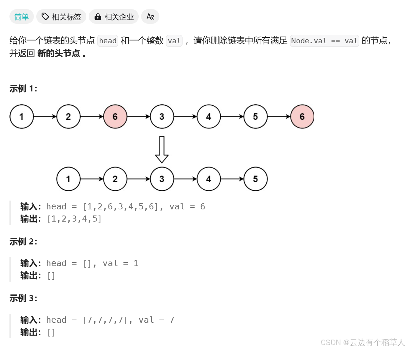
思路:
创建一个新链表(newhead,newtail),遍历原链表,把不等于 val 的结点尾插到新链表中。
/*** Definition for singly-linked list.* struct ListNode {*     int val;*     struct ListNode *next;* };*/
typedef struct ListNode ListNode;
struct ListNode* removeElements(struct ListNode* head, int val) {//创建新链表ListNode* newhead;ListNode* newtail;newhead=newtail=NULL;//遍历数组ListNode* pcur=head;while(pcur){if(pcur->val!=val){//又分两种情况,链表为空,不为空if(newhead==NULL){newtail=newhead=pcur;}else{newtail->next=pcur;newtail=newtail->next;}}pcur=pcur->next;}//[7,7,7,7,7],val=7 ,这种情况下,newtail=NULL,newtail->next=NULL,此时newtail不能解引用,所以加上if条件if(newtail)               newtail->next=NULL;return newhead;
}
注意:
当原链表为空时,newhead = newtail = pcur;
在实例中,最后一个5结点被尾插到新链表中时,5结点的next指针指向的仍然是后面的6结点,所以最后返回的时候结果里面含有6,所以我们把最后一个等于val结点的next指针指向NULL即可!
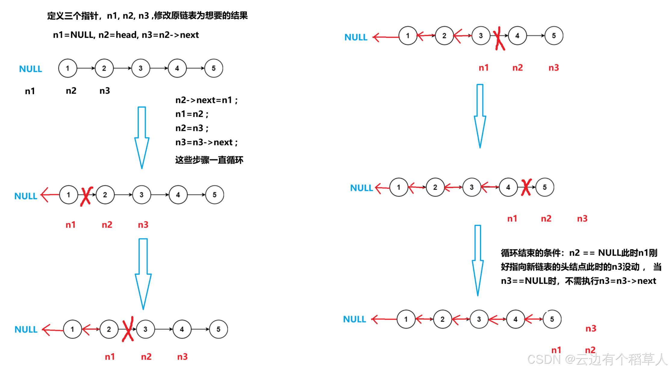
2、反转链表
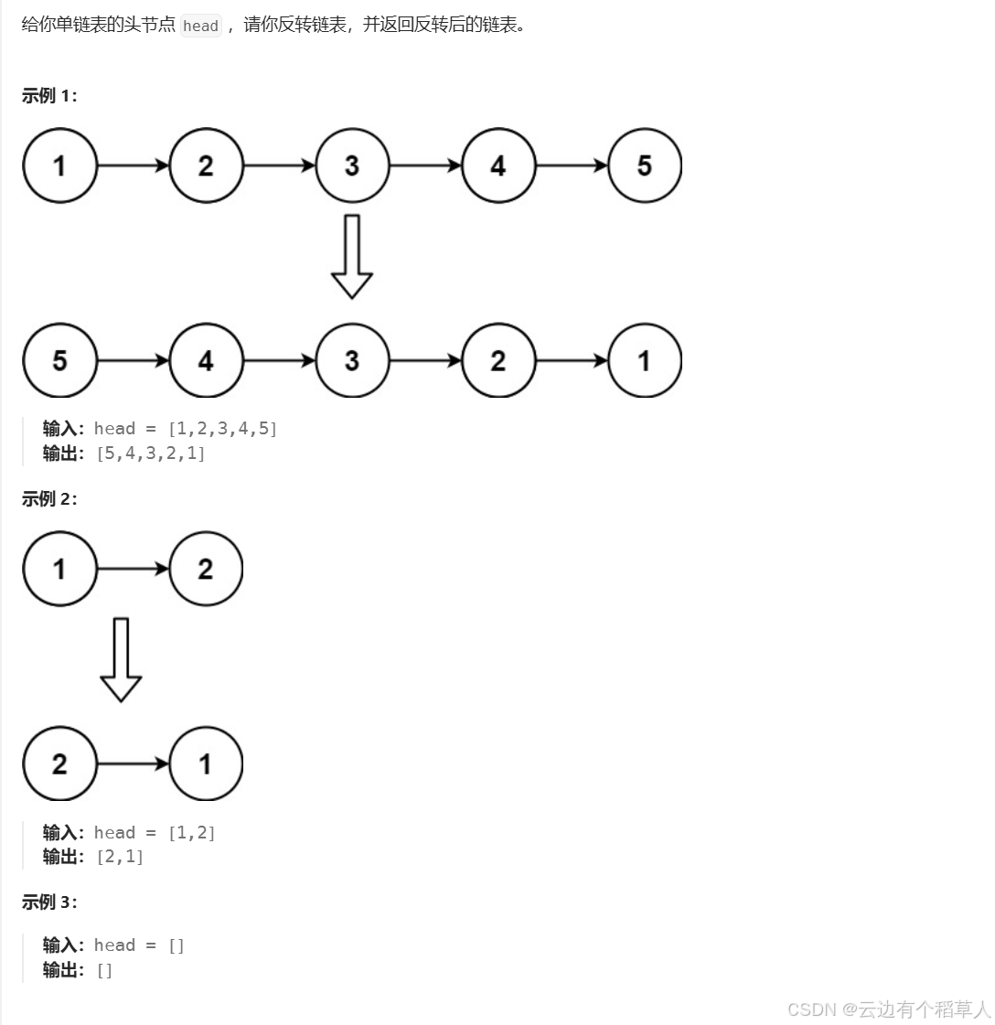
新奇思路:
/*** Definition for singly-linked list.* struct ListNode {* int val;* struct ListNode *next;* };*/typedef struct ListNode ListNode;
struct ListNode* reverseList(struct ListNode* head) {//链表也有可能是空链表if(head==NULL){return head;}//定义三个指针变量ListNode* n1,*n2,*n3;n1=NULL;n2=head;n3=n2->next;while(n2){n2->next=n1;n1=n2;n2=n3;if(n3)n3=n3->next;}return n1;
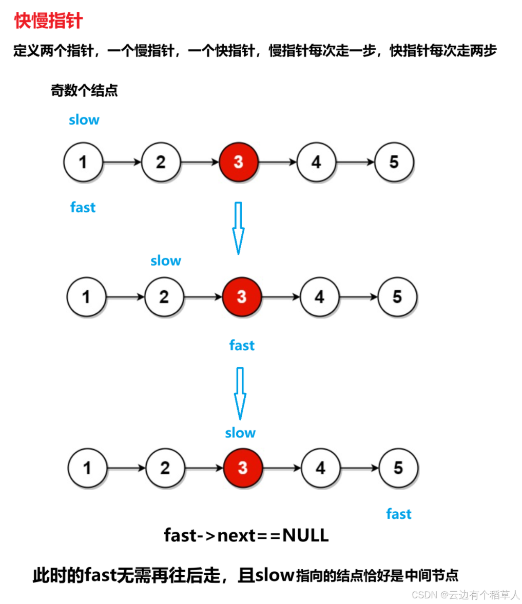
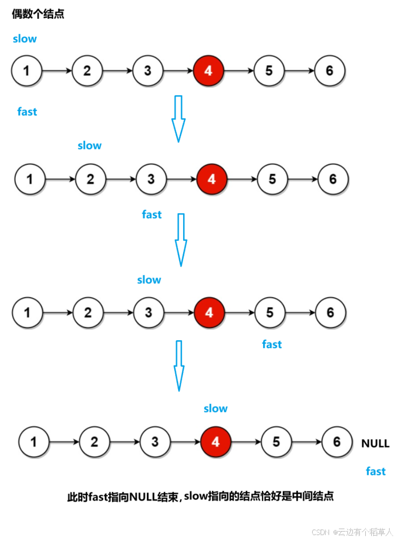
}3、链表的中间节点
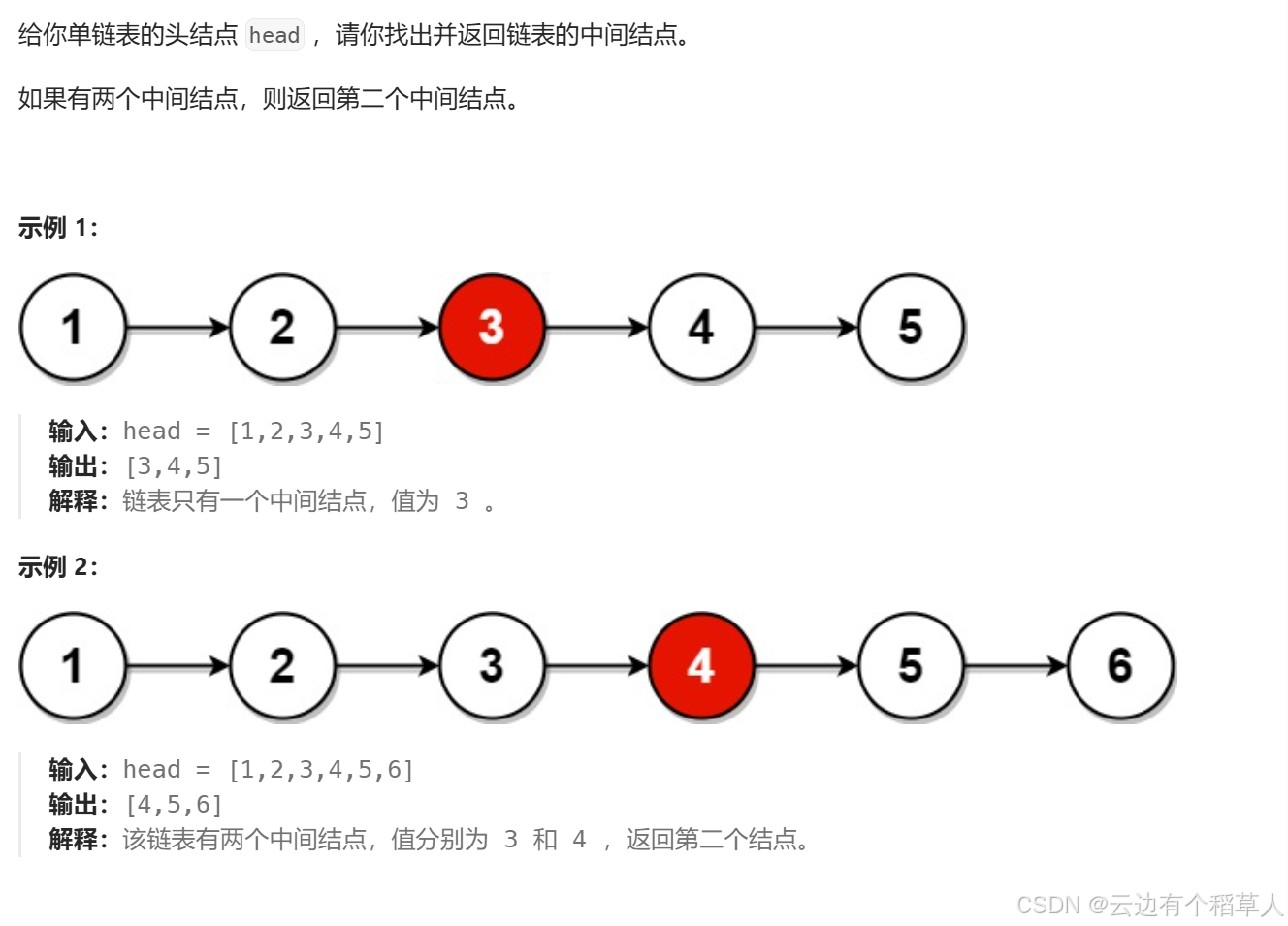
思路:
奇数个结点
偶数个结点
/*** Definition for singly-linked list.* struct ListNode {*     int val;*     struct ListNode *next;* };*/typedef struct ListNode ListNode;
struct ListNode* middleNode(struct ListNode* head) {ListNode* slow=head;ListNode* fast=head;//while(fast->next&&fast)错误,不可互换顺序,当为偶数个结点时,fast==NULL循环结束,但是while循环内会先判断fast->next,空指针不能解引用,会报错while(fast&&fast->next){//慢指针每次走一步//快指针每次走两步slow=slow->next;fast=fast->next->next;}//此时slow指向的结点恰好是中间结点return slow;
}
快慢指针为什么可以找到中间结点?(快慢指针的原理)
慢指针每次走一步,快指针每次走两步,当快指针走到链表的尾结点时,假设链表的长度为n,快指针走的路程是慢指针的两倍,2*慢=快,即慢指针走的路程是n/2。
4、合并两个有序链表
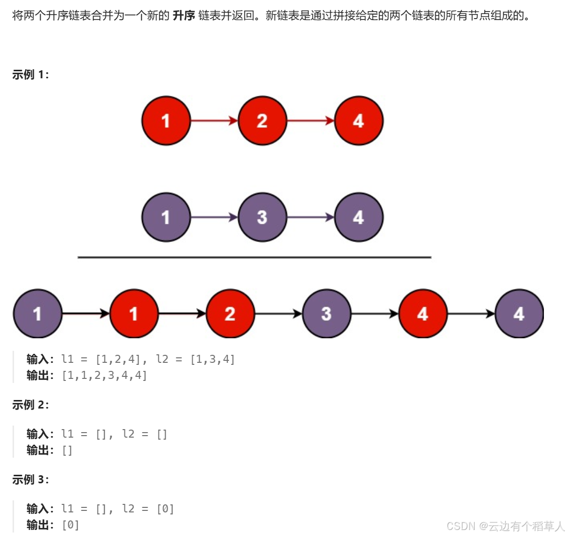
思路:
创建一个新链表,newhead,newtail 指向新链表的头结点,定义两个指针分别指向原链表的头结点,两个指针指向的数据比较大小,谁小谁尾插到新链表里面。思路清晰,不过要注意很多细节,直接上代码:
/*** Definition for singly-linked list.* struct ListNode {*     int val;*     struct ListNode *next;* };*/
typedef struct ListNode ListNode;
struct ListNode* mergeTwoLists(struct ListNode* list1, struct ListNode* list2) {//处理原链表为空链表的情况if(list1==NULL){return list2;}if(list2==NULL){return list1;}//创建一个新链表ListNode* newhead=NULL;ListNode* newtail=NULL;//创建两个指针分别指向两个链表的头结点来遍历原链表ListNode* l1=list1;ListNode* l2=list2;while(l1&&l2){if(l1->val<l2->val){//l1尾插到新链表if(newtail==NULL){newtail=newhead=l1;}else{newtail->next=l1;newtail=newtail->next;}l1=l1->next;}else{//l2尾插到新链表if(newhead==NULL){newtail=newhead=l2;}else{newtail->next=l2;newtail=newtail->next;}l2=l2->next;}}//出循环,要么l1==NULL,要么l2==NULLif(l1)newtail->next=l1;  想想这里为啥不用while循环?if(l2)newtail->next=l2;return newhead;
}
//优化过后,申请一个不为空的链表,就无需再判断新链表是否为空,最后不要忘记free
/*** Definition for singly-linked list.* struct ListNode {* int val;* struct ListNode *next;* };*/typedef struct ListNode ListNode;
struct ListNode* mergeTwoLists(struct ListNode* list1, struct ListNode* list2) {//链表为空的情况if(list1==NULL){return list2;}if(list2==NULL){return list1;}//创建一个新链表ListNode* newhead,*newtail;newhead=newtail=(ListNode*)malloc(sizeof(ListNode));//定义两个指针来遍历数组ListNode* l1=list1;ListNode* l2=list2;while(l1&&l2){if(l1->val<l2->val){newtail->next=l1;l1=l1->next;newtail=newtail->next;}else{newtail->next=l2;l2=l2->next;newtail=newtail->next;}}if(l1)newtail->next=l1;if(l2)newtail->next=l2;ListNode* ret=newhead->next;free(newhead);newhead=NULL;return ret;}完—
Relaxing Time!!!
———————————————— 天气之子·幻 ————————————————
天气之子·幻_TypeD_高音质在线试听_天气之子·幻歌词|歌曲下载_酷狗音乐酷狗音乐为您提供由TypeD演唱的高清音质无损天气之子·幻mp3在线听,听天气之子·幻,只来酷狗音乐!![]() https://t4.kugou.com/song.html?id=b43Kh7aCPV2
https://t4.kugou.com/song.html?id=b43Kh7aCPV2

至此结束——
再见——