西丽做网站优帮云首页推荐
25年4月来自清华、北大、Galbot、上海AI实验室、上海姚期智研究院、南京大学和同济大学的论文“Unleashing Humanoid Reaching Potential via Real-world-Ready Skill Space”。
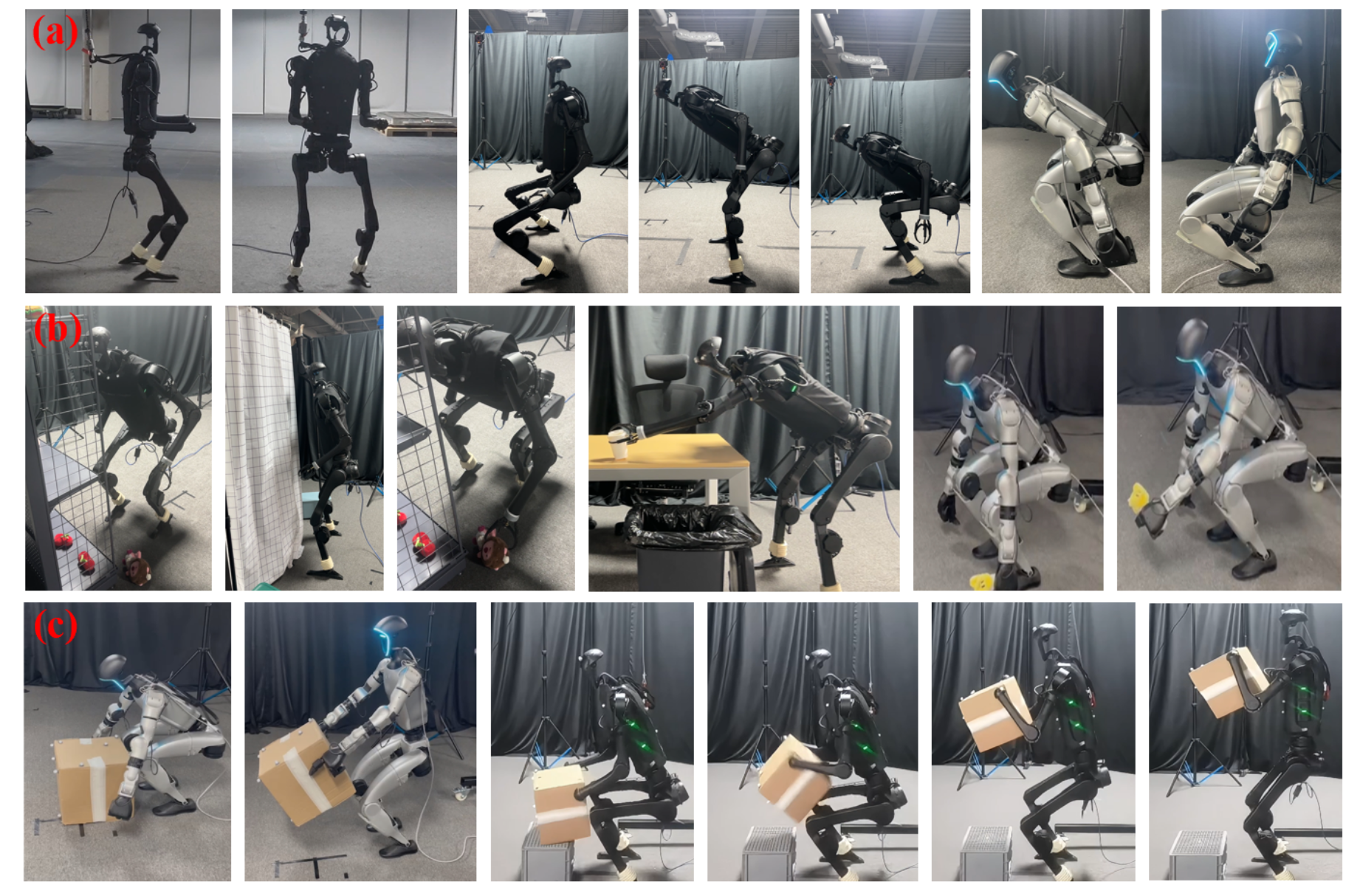
人类在三维世界中拥有巨大的可达空间,能够与不同高度和距离的物体进行交互。然而,在人形机器人上实现如此大空间的可达性是一个复杂的全身控制问题,需要机器人同时掌握多种技能,包括基定位和重定向、高度和身体姿势调整以及末端执行器位姿控制。从头学习通常会导致优化困难和 sim2real 迁移性差。为了应对这一挑战,采用现实世界现成的技能空间 (R2S2)。该方法始于一个设计的技能库,其中包含现实世界现成的原始技能。通过对单个技能的调整和 sim2real 评估来确保最佳性能和稳健的 sim2real 迁移。然后,这些技能被集成到一个统一的潜空间中,作为结构化的先验,以高效且 sim2real 可迁移的方式帮助任务执行。经过训练可以从该空间采样技能的高级规划器使机器人能够完成现实世界的目标达成任务。演示零样本 sim2real 迁移,并在多个具有挑战性的目标达成场景中验证 R2S2,包括点触摸和盒子拾取,如图所示。
人形机器人学习。强化学习 (RL) 策略在近期的人形机器人学习中取得了巨大进步。运动研究 [23、24、25、26、27、28、29、30、31] 旨在为双足人形机器人提供以稳定和敏捷的方式穿越不同地形的能力。但这些研究通常仅关注人形机器人的下半身,而忽略了它们全身的触及和交互潜力。基于学习的人形全身控制 [14、15、16、17、19、20、32、33、34、35] 最近展示了新功能并突破了人形机器人的界限。数据驱动的运动跟踪方法 [14、15、32、19、20、33、34] 富有表现力地模仿人类运动,允许人与人之间的遥操作。Zhang [16] 将类人机器人的全身控制表述为顺序接触,并提出了基于接触的 WBC 框架。然而,现有研究要么采取相对中性的身体姿势 [16, 17],要么缺乏用于实际任务完成的规划模块 [35]。如何使类人机器人具备人类级别的目标达成能力仍未得到充分探索。
技能空间学习。在基于物理的角色动画中,通常会学习技能空间 [36, 37, 38, 39, 40, 41, 42, 43, 44, 45, 46],以重用来自动作捕捉数据集的运动先验。运动模仿 [37, 39, 40, 41, 42, 46, 47] 或对抗学习 [36, 43, 44, 45] 用于形成技能潜空间,然后可以通过解码器将采样的潜变量转换为动作。对于高级任务,特定任务的规划器会学习重用预构建潜空间中的技能,从而更高效、更自然地完成任务。尽管技能空间学习在基于物理的角色动画 [38, 48, 49] 中取得了巨大成功,但由于缺乏高质量的类人运动数据集以及 sim2real 的难度,将这种范式迁移到现实世界的人形机器人仍面临挑战。与这些研究不同,为了确保现实世界的稳定性,本文从 sim2real 评估的(可用于现实世界的)原始技能(而非动作捕捉数据)中学习技能空间。
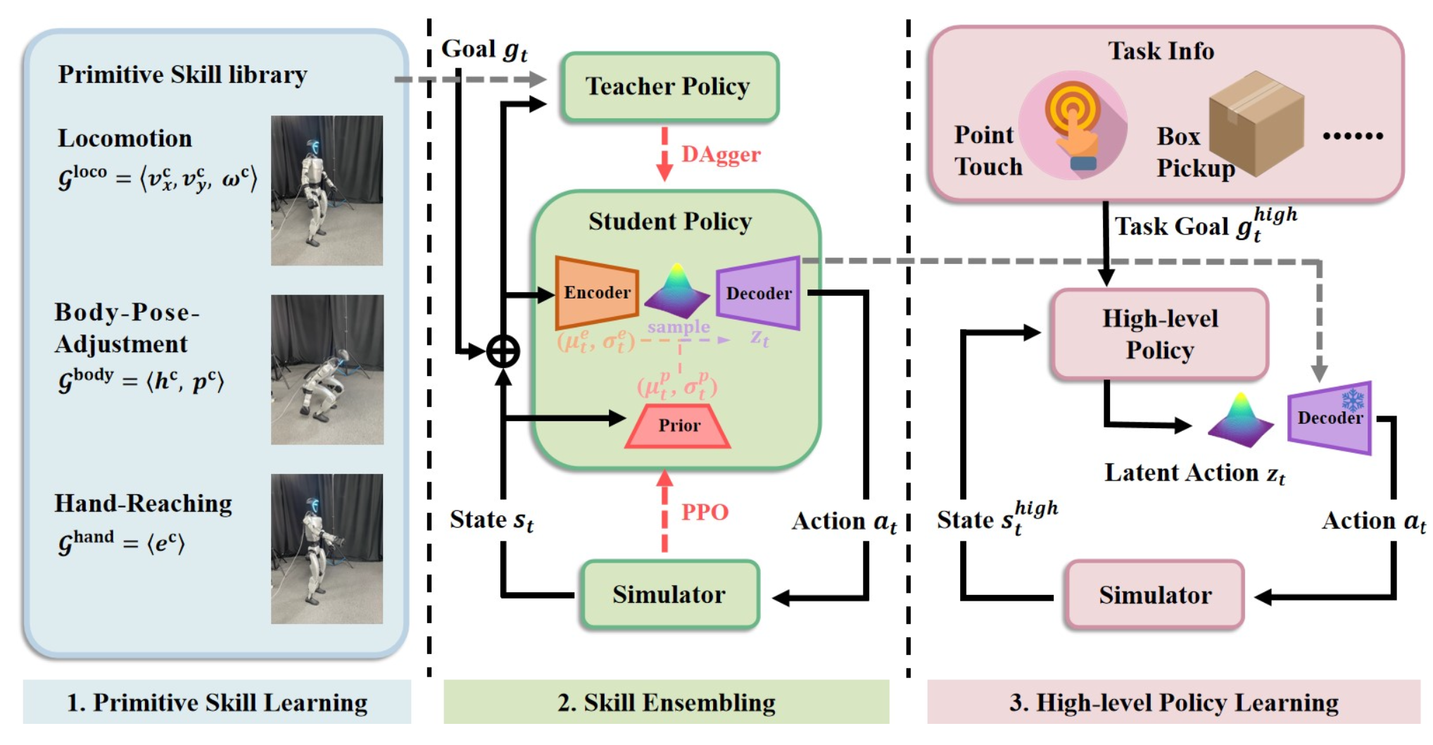
首先,构建一个包含 n 个共享且易于定义基于强化学习的原始技能库 {πprim_1,…,πprim_n},其中每个技能 πprim_i 都经过单独调优,并进行 sim2real 评估(可用于实际应用)。然后,将这些技能集成并编码,将学习过程 (IL) 和强化学习 (RL) 结合成一个集成学生策略 πensem,并包含一个潜技能 z 空间。学习的技能空间包含各种可用于实际应用的运动技能,作为技能先验,并以 sim2real 可迁移的方式辅助任务执行。利用学习的技能 z 空间,训练高级规划器 πplan 来采样潜技能,从而完成实际任务。该流程如图所示。用 PPO [50] 进行所有策略训练,使用域随机化进行 sim2real 迁移,并使用 Isaac Gym [51] 进行模拟。
原始技能库
为了释放人形机器人的伸展潜能,设计原始技能库 {πprim_1,…,πprim_n},涵盖运动、身体姿势调整(例如改变身高、弯腰)和伸手。每个技能都经过单独调优和 sim2real 评估,以最大限度地提升其能力和现实世界的稳定性。
原始技能可以理解为目标条件化的强化学习策略 πprim : Gprim × Sprim → Aprim,其中 Gprim 包含指定技能目标的目标命令 g_t;Sprim 包含机器人在每个时间步 t 的本体感受观察和历史动作信息 s_t = [ω_t, gr_t, q_t, q ̇_t, a_t−1],其中 ω_t、gr_t、q_t、q ̇_t、a_t−1 分别为基准坐标系中的角速度、投影重力、身体部位自由度位置、身体部位自由度速度和最后一帧的低级动作。值得注意的是,对于 q_t、q ̇_t、a_t−1,每个策略仅将相关身体部位信息作为不同技能的观察值。Aprim 包含机器人身体部位动作(PD 目标)aprim,该动作被输入到 PD 控制器中进行扭矩计算。aprim 仅控制每个技能的相应身体部位,其他关节是固定的。它们的训练奖励可以写成:r_prim = r_command + r_behavior + r_regularization,其中 r_task 表示技能命令跟踪目标,r_behavior 描述针对 sim2real 稳定性的技能特定行为约束,r_regularization 是与技能无关的正则化。
对于运动,Gloco = ⟨v_xc , v_yc , ωc⟩ 驱动人形机器人在机器人基框架内追踪机器人基所需的线速度和角速度。为了约束运动行为并复制类似人类的双足步态,将每只脚的运动建模为摆动和站立阶段的交替序列,并引入周期性奖励框架。
对于身体姿势调整,Gbody = ⟨hc , pc⟩ 跟踪全局坐标系中的基准高度和俯仰角。对于这样的技能,运动学和动力学对称性对于现实世界的稳定性至关重要。
对于伸手动作,Ghand = ⟨ec⟩ 跟踪机器人局部坐标系中目标末端执行器的六维姿态。手臂对于 sim2real 部署来说相对容易,因此没有专门为此技能设计任何 r_behavior。
面向现实世界的技能空间
给定面向现实世界的原始技能 {πprim_1,…,πprim_n},直接尝试将这些原始技能复用到不同的任务中,就是直接在其主要任务空间中进行规划。但这些技能空间实际上不足以构成一个实用的技能空间。由于训练分散,原始技能之间彼此不可见。不同技能之间的协调(例如,上半身够到物体的同时下半身下蹲)和过渡(例如,下半身从运动到身体姿势调整)属于分布外问题。简单地连接不同身体部位的动作或从运动技能切换到身体姿势调整技能会导致机器人不稳定,甚至跌倒。如果没有无缝的协调和过渡,技能空间就不完整,无法完成实际任务。此外,原始技能任务空间(v_xc、v_yc、ωc 用于运动,hc、pc 用于身体姿势调整,ec 用于伸手)的不匹配对于高级规划而言效率低下。
为了解决这些问题,本文提出训练一个集成学生策略 πensem(a_t|s_t,g_t),并引入变分信息瓶颈来集成不同的技能。“集成”不仅意味着模仿不同的原始技能,还意味着学习它们的协调和过渡。在技能集成过程中,不同的技能被编码到潜技能 z 空间中,然后解码为每个关节的动作。
在线模仿学习方法(例如 DAgger [53])通常用于从教师策略到学生策略的技能提炼。然而,仅仅依靠模仿学习无法为学生策略提供超越教师策略的新功能(例如,不同技能之间的协调和转换)。因此,将模仿学习和强化学习结合起来,将 IL 损失和 RL 损失结合起来。IL(在设置中是 DAgger)从多个教师策略中提炼出可用于现实世界的技能先验。在此基础上,RL(在设置中是 PPO)进一步鼓励策略学习新行为,实现无缝过渡和协调。与单独训练原始技能不同,从两个方面修改训练环境:1)同时为不同的身体部位发送目标命令(例如,策略需要在行走的同时跟踪目标手的 6D 姿势),以模拟技能协调性;2)允许某个身体部位的技能在一个回合中从一个技能过渡到另一个技能,以模拟技能过渡。形式化地讲,在每个时间步 t,两个原始技能 {πlower_t, πupper_t},πlower_t ∈ {πloco_t, πbody_t} 和 πupper_t ∈ {πhand},作为针对不同身体部位的教师策略,一个针对下半身,另一个针对上半身。学生策略目标 g_t 中包含一个技能指标,用于指示激活哪个教师策略。当发生转换时,令 πlower_t+1 ̸= πlower_t。这样,不同技能之间所有可能的协调和转换都包含在学生策略中。
奖励函数如下:

其中

对于 L_PPO,只需将原始技能训练阶段定义的奖励项 πlower_t 和 πupper_t 组合即可。学生策略无需任何额外的奖励项即可成功学习协调和过渡技能。虽然协调和过渡是在此阶段新学到的,但从教师策略中继承的技能先验知识可以起到良好的热身作用,并使新技能能够迁移到真实世界。
虽然学生策略可以集成多种原始技能,但由于缺乏统一的技能表征,不匹配的技能空间会阻碍高效的高级规划。为了缓解这个问题,采用一个带有条件变分信息瓶颈的编码器-解码器框架。使用变分编码器 E(z_t|s_t, g_t) = N (z_t; μe(s_t, g_t), σe(s_t, g_t)) 来建模以当前状态和目标为条件的潜编码。相应的解码器 D(a_t|s_t, z_t) 将采样的潜编码映射到以状态为条件的动作。受 [40] 的启发,引入一个可学习的条件先验 P(z_t|s_t) = N (z_t; μp(s_t), σp(s_t)) 来捕捉基于状态的动作分布,而不是假设潜空间上存在一个固定的单峰高斯结构,因为机器人的动作分布在不同状态下应该存在显著差异。因此,集成学生策略可以表述为 πensem =△(E,D,P)。训练过程中的总损失 πensem可以写成:

其中


基于已学习的潜技能空间,训练特定任务的高级规划器 πplan(z_t |shigh_t,ghigh_t),以针对不同的目标达成任务选择潜技能嵌入。πplan 的动作现在位于潜空间 z_t 中。采样的 z_t 通过冻结解码器 D 解码为每个关节的动作。训练奖励可以写成:r_plan = r_task + r_regularization,其中 r_task 是任务执行目标,r_regularization 是在技能库构建阶段引入的与技能无关的正则化奖励。重用 r_regularization 可以增强运动稳定性。
人形机器人的触及问题定义为:给定一个目标触及状态 [xyω_root, xyz_hand],机器人能否成功触及该状态。xyω_root 是机器人根的水平位置和方向。xyz_hand 是当 xyω_root 固定时,机器人手部能够触及的三维位置。由于大多数现有机器人都具备全向运动能力,并且已经能够满足平面地面上任意 xyω_root 的触及要求,因此主要比较机器人触及任意给定 xyz_hand 的能力。
如何释放人形机器人的伸展潜能尚未得到充分探索。相关研究成果寥寥无几。主要将方法与近期两篇专注于在与实验相同的硬件(Unitree H1)上进行全身控制的研究成果进行比较:
• ExBody [14]。该研究将运动目标分解为运动目标和表达目标,运动目标包括对机器人基座的指令,例如速度、滚动、俯仰和基座高度。在仿真中复现该方法,并将其部署到硬件上。
• HUGWBC [28]。该研究提出一种统一的全身控制器,可以实现多种运动并调整身体姿势。由于代码不可用,根据其原始论文中的姿势调整参数计算可达空间。
• 本文方法 w/ohc,pc。消融基元技能的任务空间,以评估每个部分对可达空间的贡献。
对于真实世界现成的技能空间,其评估如下。
在真实实验环境中,评估 R2S2 的每种设计如何帮助完成两个目标达成任务:点触碰和拾取箱子。对于点触碰,在机器人前方 2m × 2m 的方格内随机设置一个点,高度范围为 0.1 米至 2.0 米。要求人形机器人用特定的手触摸该点。对于拾取箱子,将箱子随机放置在机器人前方 2m × 2m 的方格内,高度范围为 0.2 米至 1.2 米。要求人形机器人将箱子举到 1.4 米的高度。
在 R2S2 的不同组件上进行消融,并选择以下基准:
• 原始 PPO。实现一个原始 PPO,尝试在没有任何技能先验的情况下从头完成每个目标达成任务。
• 不带 SE(技能集成)的 R2S2。用单独的原始技能作为技能空间。在此设置中,训练一个高级规划器策略,使其直接在主任务空间中输出技能指标和命令。采用此基准主要是为了验证协调和过渡能力的重要性。
• R2S2 w/o LS(潜空间)。实现一个基于多层感知器 (MLP) 的学生策略,用于集成来自多个教师策略的技能。在此设置中,尽管原始技能已被集成(即学习协调和过渡),但高级规划策略仍然需要在不匹配的主任务空间中输出技能指标和命令才能执行任务。采用此基准来评估潜技能空间的有效性。