网站建设平台安全问题有哪些方面安阳中飞网站建设
对于开发同学来说,Spring 框架熟悉又陌生。 熟悉:开发过程中无时无刻不在使用 Spring 的知识点;陌生:对于基本理论知识疏于整理与记忆。导致很多同学面试时对于 Spring 相关的题目知其答案,但表达不够完整准确。今天展示互联网公司Java面试高频常问的100道题及解析!

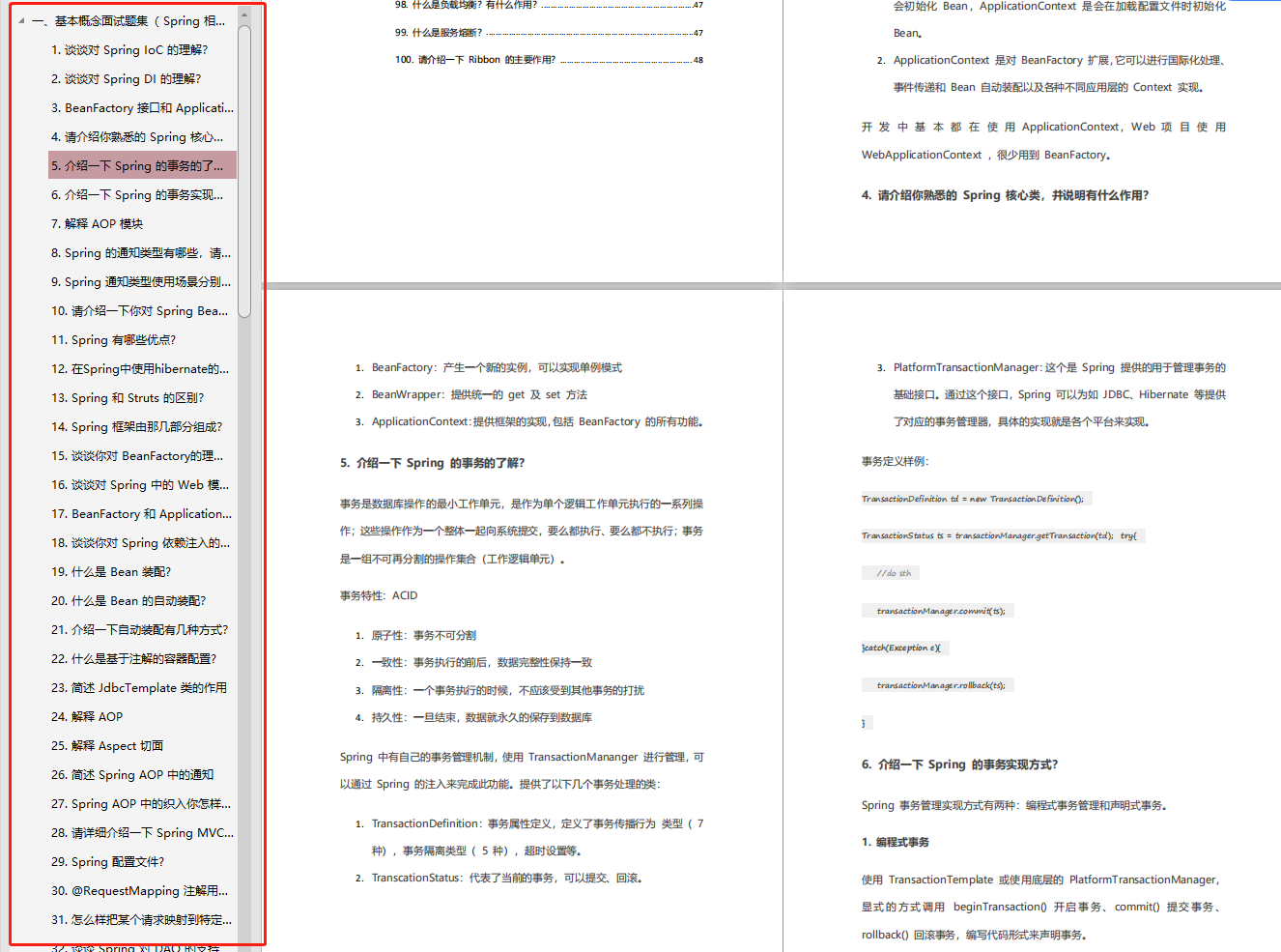
一、基本概念面试题集( Spring 相关概念梳理)
-
谈谈对 Spring IoC 的理解?
-
谈谈对 Spring DI 的理解?
-
BeanFactory 接口和 ApplicationContext 接口不同点是什么?
-
请介绍你熟悉的 Spring 核心类,并说明有什么作用?
-
介绍一下 Spring 的事务的了解?
-
介绍一下 Spring 的事务实现方式?
-
解释 AOP 模块
-
Spring 的通知类型有哪些,请简单介绍一下?
-
Spring 通知类型使用场景分别有哪些?
-
请介绍一下你对 Spring Beans 的理解?
-
Spring 有哪些优点?
-
在Spring中使用hibernate的方法步骤
-
Spring 和 Struts 的区别?
-
Spring 框架由那几部分组成?
-
谈谈你对 BeanFactory的理解,BeanFactory 实现举例
-
谈谈对 Spring 中的 Web 模块的理解
-
BeanFactory 和 Application contexts 有什么区别?
-
谈谈你对 Spring 依赖注入的理解?
-
什么是 Bean 装配?
-
什么是 Bean 的自动装配?
-
介绍一下自动装配有几种方式?
-
什么是基于注解的容器配置?
-
简述 JdbcTemplate 类的作用
-
解释 AOP
-
解释 Aspect 切面
-
简述 Spring AOP 中的通知
-
Spring AOP 中的织入你怎样理解?
-
请详细介绍一下 Spring MVC 的流程?
-
Spring 配置文件?
-
@RequestMapping 注解用在类上面有什么作用
-
怎么样把某个请求映射到特定的方法上面
-
谈谈 Spring 对 DAO 的支持
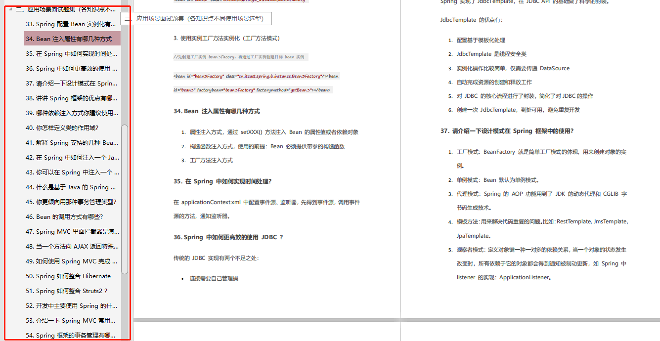
二、应用场景面试题集(各知识点不同使用场景选型)
-
Spring 配置 Bean 实例化有哪些方式?
-
Bean 注入属性有哪几种方式
-
在 Spring 中如何实现时间处理?
-
Spring 中如何更高效的使用 JDBC ?
-
请介绍一下设计模式在 Spring 框架中的使用?
-
讲讲 Spring 框架的优点有哪些?
-
哪种依赖注入方式你建议使用,构造器注入,还是 Setter 方法注入?
-
你怎样定义类的作用域?
-
解释 Spring 支持的几种 Bean 的作用域
-
在 Spring 中如何注入一个 Java 集合?
-
你可以在 Spring 中注入一个 null 和一个空字符串吗?
-
什么是基于 Java 的 Spring 注解配置? 给一些注解的例子
-
你更倾向用那种事务管理类型?
-
Bean 的调用方式有哪些?
-
Spring MVC 里面拦截器是怎么写的
-
当一个方法向 AJAX 返回特殊对象,譬如 Object、List 等,需要做什么处理?
-
如何使用 Spring MVC 完成 JSON 操作
-
Spring 如何整合 Hibernate
-
Spring 如何整合 Struts2 ?
-
开发中主要使用 Spring 的什么技术 ?
-
介绍一下 Spring MVC 常用的一些注解
-
Spring 框架的事务管理有哪些优点
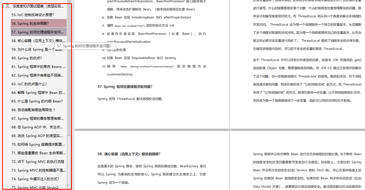
三、深度度知识面试题集(底层实现原理详解)
-
IoC 控制反转设计原理?
-
Spring 的生命周期?
-
Spring 如何处理线程并发问题?
-
核心容器(应用上下文)模块的理解?
-
为什么说 Spring 是一个容器?
-
Spring 的优点?
-
Spring 框架中的单例 Beans 是线程安全的么?
-
Spring 框架中有哪些不同类型的事件?
-
IoC 的优点是什么?
-
解释 Spring 框架中 Bean 的生命周期
-
什么是 Spring 的内部 Bean?
-
自动装配有哪些局限性 ?
-
Spring 框架的事务管理有哪些优点?
-
在 Spring AOP 中,关注点和横切关注的区别是什么?
-
说说 Spring AOP 的底层实现原理?
-
如何给 Spring 容器提供配置元数据?
-
哪些是重要的 Bean 生命周期方法? 你能重载它们吗?
-
讲下 Spring MVC 的执行流程
-
Spring MVC 的控制器是不是单例模式,如果是,有什么问题,怎么解决?
-
Spring 中循环注入的方式?
-
Spring MVC 比较 Struts2
四、拓展内容面试题集(Spring Boot 相关题集)
-
什么是 Spring Boot?
-
Spring Boot 自动配置的原理?
-
Spring Boot 读取配置文件的方式?
-
什么是微服务架构?
-
Ribbon 和 Feign 的区别?
-
Spring Cloud 断路器的作用?
-
为什么要用 Spring Boot?
-
Spring Boot 的核心配置文件有哪几个?它们的区别是什么?
-
Spring Boot 的配置文件有哪几种格式?它们有什么区别?
-
Spring Boot 的核心注解是哪个?它主要由哪几个注解组成的?
-
开启 Spring Boot 特性有哪几种方式?
-
Spring Boot 需要独立的容器运行吗?
-
运行 Spring Boot 有哪几种方式?
-
你如何理解 Spring Boot 中的 Starters?
-
如何在 Spring Boot 启动的时候运行一些特定的代码?
-
Spring Boot 有哪几种读取配置的方式?
-
Spring Boot 实现热部署有哪几种方式?
-
Spring Boot 多套不同环境如何配置?
-
Spring Boot 可以兼容老 Spring 项目吗,如何做?
-
什么是 Spring Cloud?
-
介绍一下 Spring Cloud 常用的组件?
-
Spring Cloud 如何实现服务注册的?
-
什么是负载均衡?有什么作用?
-
什么是服务熔断?
-
请介绍一下 Ribbon 的主要作用?
总结
“做程序员,圈子和学习最重要”因为有有了圈子可以让你少走弯路,扩宽人脉,扩展思路,学习他人的一些经验及学习方法!
Java后端面试专题文档
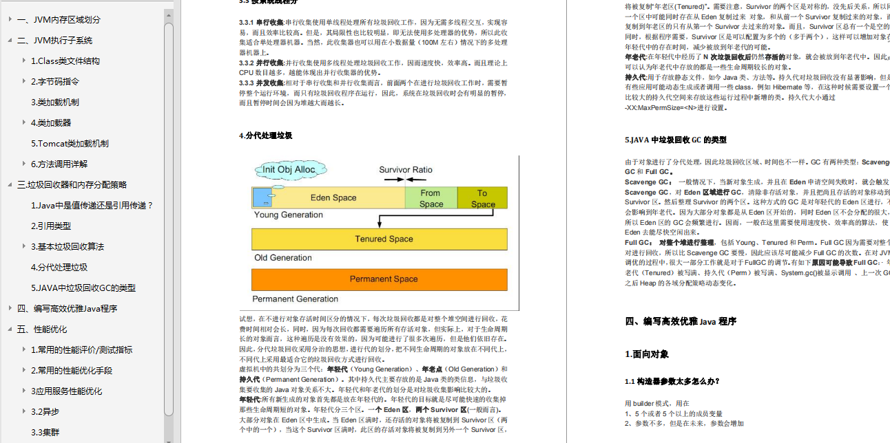
Java虚拟机(JVM)及性能优化
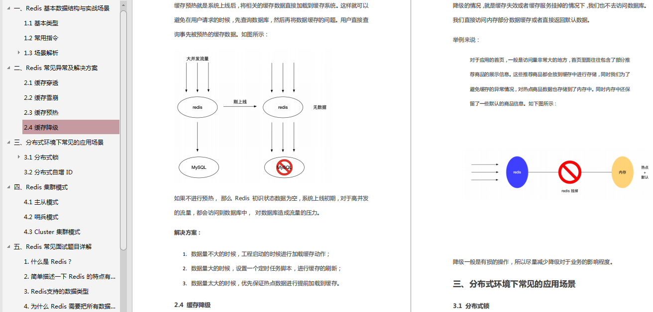
Redis学习经验笔记
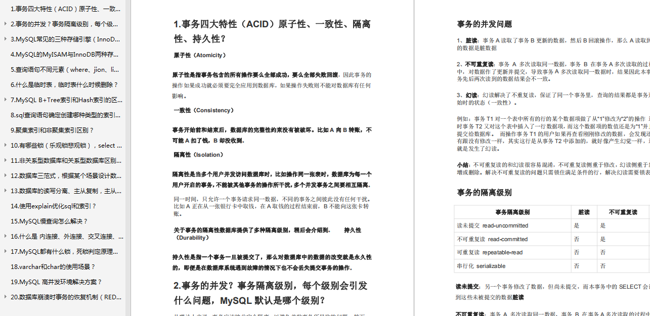
MySQL高性能数据库
设计模式

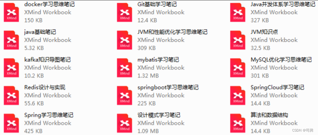
Java后端学习笔记导图
以上这些Java秋招高频面试全解析及后端技术学习经验笔记和学习导图