郑州网站运营实力乐云seowordpress有广告插件下载
-
服务器安装环境
将.net core程序部署到IIS总体需要经过以下3个大步骤,其中在IIS上配置网站有些比较繁琐,我都会逐一给出详细步骤。
<1>安装IIS和.NetCORE运行时程序
<2>以文件的形式发布.NETCORE程序到指定目录
<3>IIS上面建立网站并配置好网站设置
一.服务器安装环境,
安装IIS和.net core运行时程序
部署.net core程序首先要确保你服务器上的IIS环境要安装好,确保IIS安装好了后,还需要安装.net core的运行时,运行时的程序文件可以在官网下载最新版本安装。

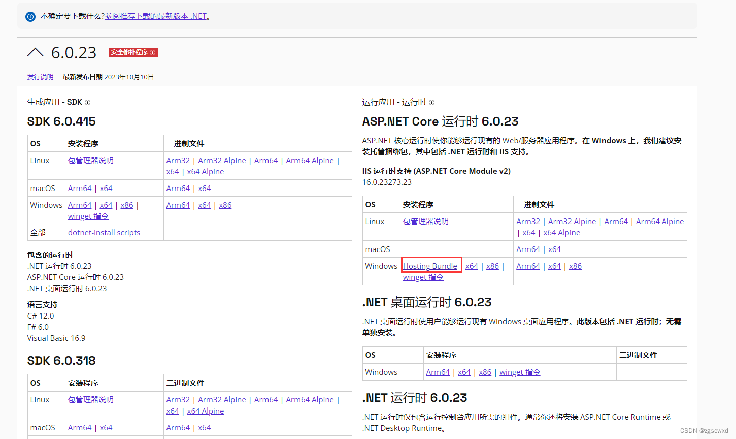
选择好版本后,点击去,找到Core运行时的支持:IIS runtime support,里面的Hosting Bundle(托管捆绑包)下载,并安装.NET Core Windows Server Hosting
部署asp.net core web api项目需要安装环境,IIS默认是不支持的,支持环境需要安装net core运行时: dotnet-hosting-7.0.12-win.exe,.net core项目不是由iis工作进程(w3wp.exe)托管,需要先下载dotnet-hosting-7.0.12-win.exe

.net core环境运行时,安装好了后,在IIS上模块里面看到AspNetCoreModuleV2模块,表示安装成功


基本环境配置好了后,下面该发布.net core 程序了。
二.先基本的发布
-
操作:右击web项目的《发布》按钮。选文件
以文件的形式发布.net core程序到指定目录
三.上传发布文件
在服务器上新建文件夹,用于放置程序。将在本地发布的项目,拷贝到服务器上的文件夹里。

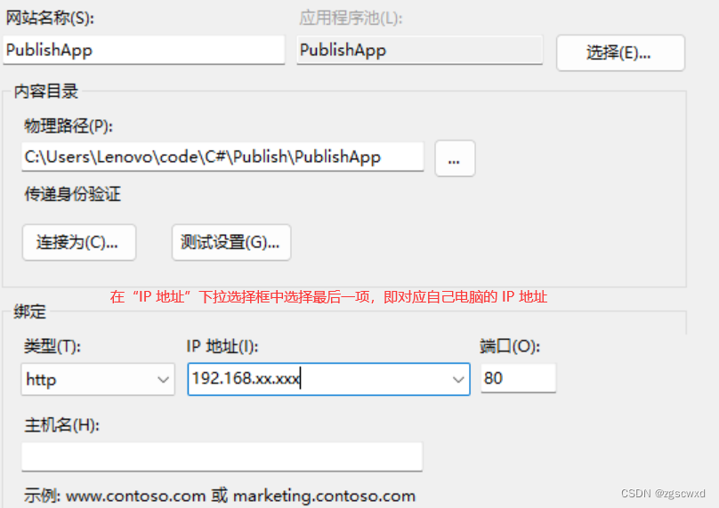
四.在IIS上添加站点
右击=》添加网站,配置完确认即可:指定网站名称,指定网站承载程序的路径,指定IP+端口


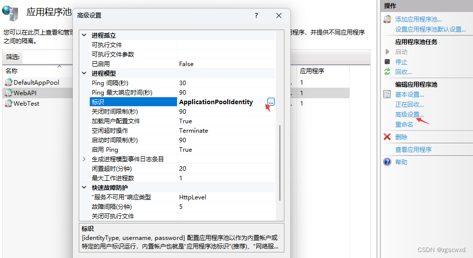
五.配置程序池
点击“应用程序池”,找到与自己的网站同名的应用程序,右键选择“基本设置”,在“.NET CLR 版本”下拉选择框中选择“无托管代码”

对于使用数据库的应用程序,需要设置标识以访问数据库。 再次右键选择“高级设置”,选择“进程模型” > “标识”,点击右边的按钮
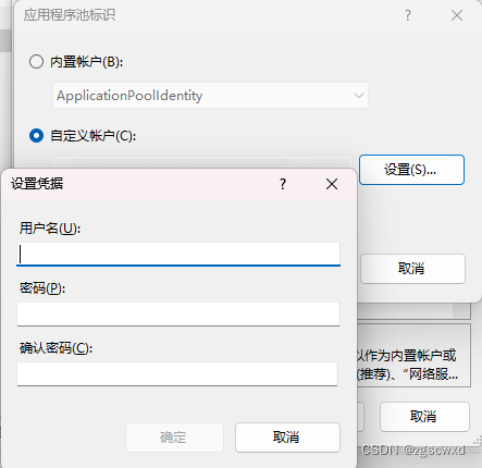
选择“自定义账户”,点击“设置”。使用 Windows 身份验证的数据库,应输入电脑的用户名及密码;使用数据库身份验证的数据库,应输入其账号对应的用户名及密码。点击“确定”。
IIS标识
本地系统(Local System): 具有高特权且有权访问网络资源的受信任帐户。
网络服务(Network Service): 用于运行标准最小特权服务的受限或受限服务帐户。 此帐户的权限比本地系统帐户少。 此帐户有权访问网络资源。
本地服务(Local Service): 与网络服务类似且旨在运行标准最小特权服务的受限或受限服务帐户。 此帐户无法访问网络资源。
ApplicationPoolIdentity: 创建新的 应用程序池 时,IIS 会创建一个虚拟帐户,该帐户的名称为新 应用程序池并且在此帐户下运行 应用程序池 工作进程。 这也是最小特权帐户。
自定义帐户(Custom account): 除了这些内置帐户之外,您还可以通过指定用户名和密码来使用自定义帐户。