好一点网站建设公司上海大型网站
在如今逐渐老龄化的社会中,老年人对更好的护理服务需求不断增加。科技的进步使得陪护小程序系统源码成为提供优质服务的重要途径之一。本文将从运营角度探讨如何优化陪护小程序系统源码,提升长者护理服务的质量。
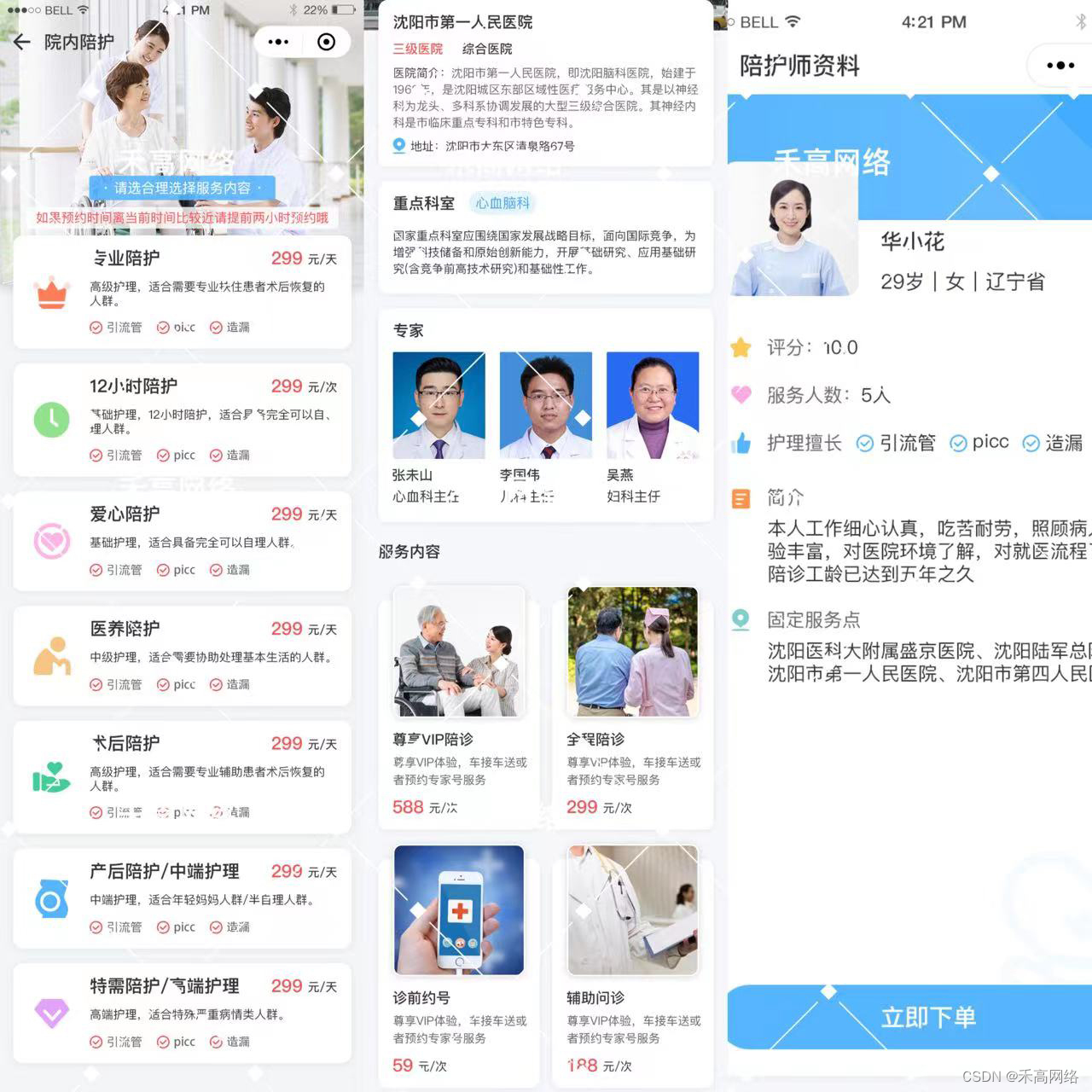
首先,我们需要对软件的设计和用户体验进行全面优化。陪护小程序系统源码的界面应简洁明了,易于操作,以方便长者和护理人员使用。同时,还应提供咨询和反馈渠道,以方便长者或其家属提出问题和意见。这些问题和意见可及时反馈给系统开发人员或客服人员,进一步改进产品。
其次,护理人员的培训和管理至关重要。首先,护理人员应接受全面的培训,包括沟通技巧和设备操作技能。其次,定期对护理人员进行业绩考核,并关注原因和统计评估,实现有效的员工管理。利用考核结果激励护理人员,并通过奖励等方式提高护理人员的积极性。
另外,优化开发团队的协作也是至关重要的。良好的协作能够加快开发进度,提高产品质量。跨部门沟通、信息共享和项目管理等都是促进协作和提升团队效率的重要因素。通过定期会议、项目管理工具、信息共享和良好沟通等实践,可以有效协调不同团队的工作,从而大幅提升整体项目开发周期和质量。
综上所述,在提供高质量护理服务的过程中,陪护小程序系统源码起着至关重要的作用。通过优化设计、完善管理和加强团队协作,我们能够为长者提供更加舒适、贴心的生活。这不仅让长者感到更加关爱,也体现了科技在老年护理领域的巨大影响力。